PyTorch: How to Train and Optimize A Neural Network in 10 Minutes

Deep learning might seem like a challenging field to newcomers, but it’s gotten easier over the years due to amazing libraries and community. PyTorch library for Python is no exception, and it allows you to train deep learning models from scratch on any dataset.

Sometimes it’s easier to visualize deep learning models – you can do so with these 3 examples for visualizing PyTorch neural networks.

In this article, you’ll get a hands-on experience with PyTorch by coding your first neural network from scratch and optimizing it. For the sake of speed, the network will be trained on a small Iris dataset, but you can always modify the model to fit your data.

Want to use Keras in R? Follow this guide to build a handwritten digit classifier.

Table of contents:

• How to Load Data with PyTorch Data Loaders
• Train Your First Neural Network with PyTorch
• How to Optimize Your Neural Network Models in PyTorch
• Summing up Model Training & Optimization in PyTorch

How to Load Data with PyTorch Data Loaders

First things first, we need a way to load the dataset. You could go as simple as loading a CSV file and converting it to a PyTorch Tensor object, but this approach isn’t optimal for bigger datasets. That’s the reason why we’ll use PyTorch DataLoader module, which will allow loading data in batches.

We still have to load the dataset with Python, so here’s a code snippet for all the library imports and the dataset:

import warnings
warnings.filterwarnings("ignore")

import numpy as np
import pandas as pd
import torch
import torch.nn as nn
import torch.nn.functional as F
from torch.utils.data import DataLoader, TensorDataset
from sklearn.model_selection import train_test_split

import matplotlib.pyplot as plt
import matplotlib.gridspec as gridspec
from IPython import display
display.set_matplotlib_formats("svg")

iris = pd.read_csv("https://gist.githubusercontent.com/netj/8836201/raw/6f9306ad21398ea43cba4f7d537619d0e07d5ae3/iris.csv")
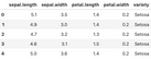
iris.head()

The head() method from Pandas shows the first five rows of the dataset:

Image 1 – Head of the Iris dataset

We want to predict the variety variable (dependent) based on the four independent variables (widths and lengths). A common way is to separate features (X) from the target variable (y), and convert both to PyTorch tensors. Keep in mind that Torch tensors should be numeric, so we’ll have to encode the target variable:

X = torch.tensor(iris.drop("variety", axis=1).values, dtype=torch.float)
y = torch.tensor(
    [0 if vty == "Setosa" else 1 if vty == "Versicolor" else 2 for vty in iris["variety"]], 
    dtype=torch.long
)

print(X.shape, y.shape)

Image 2 – Shape of the feature data tensor and target variable tensor

As you would expect, the feature tensor has a shape of 150 rows by 4 columns, while the target variable tensor has only one column with the same number of rows.

The next step you want to do when training the classification model is to train/test split. The idea is to train the model on most of the data (e.g., 80%) and evaluate it on the remainder. This way, we can make sure the high accuracies aren’t obtained because of overfitting.

With the 80:20 split, the training set will have 120 samples. We’ll load these in 12 batches with 10 samples each, and we’ll load the test set all at once. Batches aren’t really necessary for this simple of a problem, but we want to provide a workflow that’s easy for you to copy/paste between the projects:

X_train, X_test, y_train, y_test = train_test_split(X, y, train_size=0.8, random_state=42)

train_data = TensorDataset(X_train, y_train)
test_data = TensorDataset(X_test, y_test)

train_loader = DataLoader(train_data, shuffle=True, batch_size=12)
test_loader = DataLoader(test_data, batch_size=len(test_data.tensors[0]))

print("Training data batches:")
for X, y in train_loader:
    print(X.shape, y.shape)
    
print("\nTest data batches:")
for X, y in test_loader:
    print(X.shape, y.shape)

Here are the shapes of data coming in on each batch:

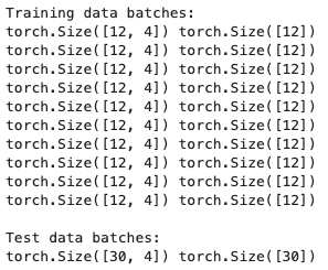
Image 3 – Batch contents

We now have the data ready for training, so next, let’s see how to build a PyTorch neural network model.

Train Your First Neural Network with PyTorch

There are multiple ways to build a neural network model in PyTorch. You could go with a simple Sequential model for this dataset, but we’ll stick to a more robust class approach.

The first model we’ll build will have a single hidden layer of 16 nodes that’s connecting the input and the output layer. Just make sure that the number of out_features on layer L-1 matches the number of in_features on layer L – otherwise, matrix multiplication won’t be possible and you’ll get an error:

class Net(nn.Module):
    def __init__(self):
        super().__init__()
        self.input = nn.Linear(in_features=4, out_features=16)
        self.hidden_1 = nn.Linear(in_features=16, out_features=16)
        self.output = nn.Linear(in_features=16, out_features=3)
        
    def forward(self, x):
        x = F.relu(self.input(x))
        x = F.relu(self.hidden_1(x))
        return self.output(x)
    
    
model = Net()
print(model)

By printing the model you get a glimpse into its architecture – there are better ways to do this but this one is adequate for today:

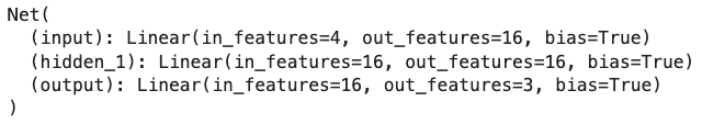
Image 4 – Model architecture

Now comes the training part. In PyTorch, you have to set the training loop manually and manually calculate the loss. The backpropagation (learning) is also handled inside the training loop.

We’ll keep track of the training and testing accuracies per epoch for visualizations later. Configuration-wise, we’ll use CrossEntropyLoss to keep track of the loss, and Adam as a gradient descent implementation:

num_epochs = 200
train_accuracies, test_accuracies = [], []

loss_function = nn.CrossEntropyLoss()
optimizer = torch.optim.Adam(params=model.parameters(), lr=0.01)

for epoch in range(num_epochs):
    # Train set
    for X, y in train_loader:
        preds = model(X)
        pred_labels = torch.argmax(preds, axis=1)
        loss = loss_function(preds, y)
        optimizer.zero_grad()
        loss.backward()
        optimizer.step()
    train_accuracies.append(
        100 * torch.mean((pred_labels == y).float()).item()
    )
    
    # Test set
    X, y = next(iter(test_loader))
    pred_labels = torch.argmax(model(X), axis=1)
    test_accuracies.append(
        100 * torch.mean((pred_labels == y).float()).item()
    )

The code shouldn’t take more than a second or so to finish, as we’re dealing with a small dataset. We have the training and testing accuracies now saved into variables, so let’s visualize them to see how the learning went:

fig = plt.figure(tight_layout=True)
gs = gridspec.GridSpec(nrows=2, ncols=1)

ax = fig.add_subplot(gs[0, 0])
ax.plot(train_accuracies)
ax.set_xlabel("Epoch")
ax.set_ylabel("Training accuracy")

ax = fig.add_subplot(gs[1, 0])
ax.plot(test_accuracies)
ax.set_xlabel("Epoch")
ax.set_ylabel("Test accuracy")

fig.align_labels()
plt.show()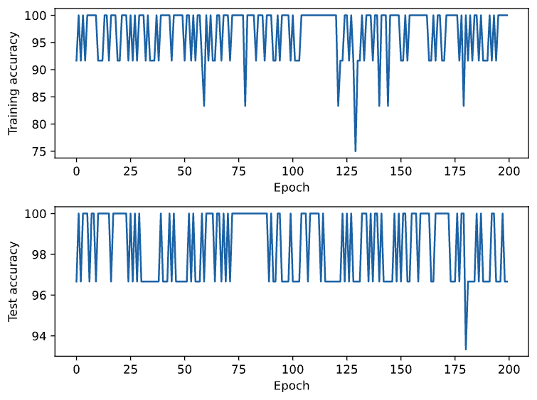

Image 5 – Training and testing accuracies per epoch

On the test set, the model is always between 97% and 100% accurate, with one exception of 94%. That’s an impressive performance for a model with only one hidden layer!

It brings the question, though – Is this the optimal model architecture? Well, we can’t possibly know before trying to optimize it. Let’s do that in the next section.

How to Optimize Your Neural Network Models in PyTorch

The optimization process boils down to trying out a couple of layer/nodes per layer combinations. The PyTorch model class allows you to introduce variability with ModuleDict(), but more on that in a bit.

Let’s start with something simpler. Just wrap the entire training logic into a train_model() function, and make sure to extract data and the model parts to the function argument. This function will do the training for us and will return the last obtained training and testing accuracy:

def train_model(train_loader, test_loader, model, lr=0.01, num_epochs=200):
    train_accuracies, test_accuracies = [], []
    loss_function = nn.CrossEntropyLoss()
    optimizer = torch.optim.Adam(params=model.parameters(), lr=lr)
    
    for epoch in range(num_epochs):
        for X, y in train_loader:
            preds = model(X)
            pred_labels = torch.argmax(preds, axis=1)
            loss = loss_function(preds, y)
            losses.append(loss.detach().numpy())
            optimizer.zero_grad()
            loss.backward()
            optimizer.step()
            
        train_accuracies.append(
            100 * torch.mean((pred_labels == y).float()).item()
        )
        
        X, y = next(iter(test_loader))
        pred_labels = torch.argmax(model(X), axis=1)
        test_accuracies.append(
            100 * torch.mean((pred_labels == y).float()).item()
        )
 
    return train_accuracies[-1], test_accuracies[-1]


train_model(train_loader, test_loader, Net())

The last line of the code snippet tests the function – you can see it works without any issues:

Image 6 – Testing the train_model() function

Onto the model now. We’ll declare a new class – Net2 – that will accept the number of layers and the number of nodes as parameters. Then, the idea is to store each layer in PyTorch ModuleDict(). This way, we can have a variable number of layers with a variable number of nodes per layer.

The rest of the class is more or less the same, but with a slightly changed code writing convention:

class Net2(nn.Module):
    def __init__(self, n_units, n_layers):
        super().__init__()
        self.n_layers = n_layers
        
        self.layers = nn.ModuleDict()
        self.layers["input"] = nn.Linear(in_features=4, out_features=n_units)
        
        for i in range(self.n_layers):
            self.layers[f"hidden_{i}"] = nn.Linear(in_features=n_units, out_features=n_units)
            
        self.layers["output"] = nn.Linear(in_features=n_units, out_features=3)
        
    def forward(self, x):
        x = self.layers["input"](x)
        
        for i in range(self.n_layers):
            x = F.relu(self.layers[f"hidden_{i}"](x))
            
        return self.layers["output"](x)

The optimization can now begin. We’ll go from 1 to 4 layers, with each layer having either 8, 16, 24, 32, 40, 48, 56, or 56 nodes. It’s quite a number of combinations, but in the end, we should see what works best for the Iris dataset:

n_layers = np.arange(1, 5)
n_units = np.arange(8, 65, 8)
train_accuracies, test_accuracies = [], []

for i in range(len(n_units)):
    for j in range(len(n_layers)):
        model = Net2(n_units=n_units[i], n_layers=n_layers[j])
        train_acc, test_acc = train_model(train_loader, test_loader, model)
        train_accuracies.append({
            "n_layers": n_layers[j],
            "n_units": n_units[i],
            "accuracy": train_acc
        })
        test_accuracies.append({
            "n_layers": n_layers[j],
            "n_units": n_units[i],
            "accuracy": test_acc
        })
        
        
train_accuracies = pd.DataFrame(train_accuracies).sort_values(by=["n_layers", "n_units"]).reset_index(drop=True)
test_accuracies = pd.DataFrame(test_accuracies).sort_values(by=["n_layers", "n_units"]).reset_index(drop=True)
test_accuracies.head()

Here are the first five accuracy reports for the test subset:

Image 7 – Head of the test accuracies dataset

The question remains: How can we extract the best model architecture? Simple – just keep the rows that have the highest accuracy on the test set:

test_accuracies[test_accuracies["accuracy"] == test_accuracies["accuracy"].max()]

Image 8 – Model architectures with the highest test accuracy

As you can see, there isn’t just one perfect combination. Multiple model architectures will result in 100% accuracy, at least on this dataset. If your dataset has thousands of testing samples, it’s unlikely that this many combinations will result in the same accuracy.

Overall, you can’t really go wrong with any of these, but it’s recommended to stick with the simplest solution that yields the best results.

Summing up Model Training & Optimization in PyTorch

Training your first neural network in PyTorch wasn’t that difficult, was it? It boils down to writing a scalable, dataset and parameter agnostic framework, which you can then copy/paste between projects. For example, you could also extract the loss function and the optimizer as function parameters, and see what happens as you change them. It’s a good idea for a homework assignment, so why don’t you give it a try?

What are your thoughts on building PyTorch neural networks? Do you prefer some other library, such as TensorFlow, and why? Please let us know in the comment section below. Also, feel welcome to move the discussion to Twitter – @appsilon – we’d love to hear your feedback.

Dive deep into image classification – Convolutional Neural Networks for seed classification.