R Quarto Tutorial – How To Create Interactive Markdown Documents

R Quarto is a next-gen version of R Markdown. The best thing is – it’s not limited to R programming language. It’s also available in Python, Julia, and Observable. In this R Quarto tutorial, we’ll stick with the most popular statistical language and create Markdown documents directly in RStudio.

With Quarto, you can easily create high-quality articles, reports, presentations, PDFs, books, Word documents, ePubs, and even entire websites. For example, the entire Hands-On Programming with R book by Garrett Grolemund is written in Quarto. Talk about scalability!

We’ll kick off today’s article by installing and configuring Quarto, and then we’ll dive into the good stuff.

R Markdown and PowerPoint presentations? Learn to create slideshows with R.

Table of contents:

• How to Get Started with R Quarto
• Render Code, Tables, and Charts with R Quarto
• How to Export R Quarto Documents
• Summary of R Quarto

How to Get Started with R Quarto

First things first, head over to their website and hit the big blue “Get Started” button. You’ll be presented with the following screen:

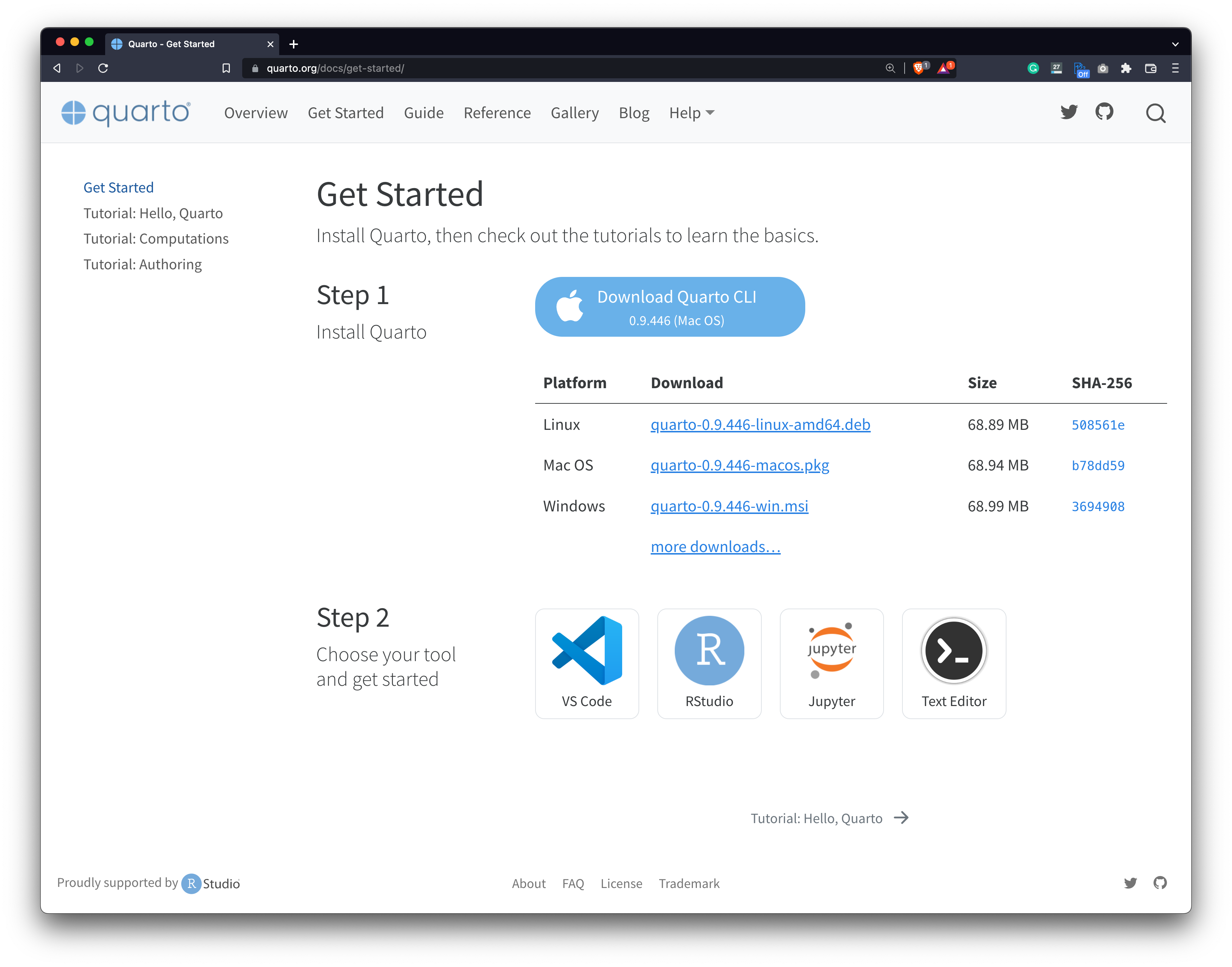
Image 1 – Getting started with R Quarto

From there, download a CLI that matches your operating system – either Windows, Linux, or Mac. We’re on macOS, and Quarto CLI downloads as a .pkg file which installs easily with a couple of mouse clicks.

Once installed, launch RStudio (you can also use VSCode or any other text editor), and create a new text file, just as it’s shown below:

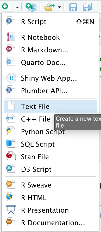
Image 2 – Creating a new text document in RStudio

Important note: Make sure to give the .qmd extension to the Quarto file. We’ve named ours quarto.qmd, for reference.

Almost there! The final step is to install two R packages – tidyverse and palmerpenguins. Install them from the R console by running the following commands:

install.packages("tidyverse")
install.packages("palmerpenguins")

And that’s it! You’re ready to create your first R Quarto document.

Render Code, Tables, and Charts with R Quarto

As with any Markdown document, a good practice is to include a YAML header to provide some context around your document. The entire header has to be demarcated by three dashes (---) on both ends.

The example below shows how to include the document title, author, and date to the YAML header of an R Quarto file:

---
title: "Quarto Demo"
author: "Appsilon"
date: "2022-5-24"
---

Once you write yours, hit the “Render” button to preview the document. It’s located in the toolbar just below the document name:

Image 3 – Toolbar for rendering R Quarto documents

Here’s what the rendered document looks like on our end:

Image 4 – Rendered R Quarto document

You can also check the “Render on Save” checkbox so you don’t have to manually render the document each time you make a change. Optionally, you can also render Quarto documents through the R console:

install.packages("quarto")
quarto::quarto_render("notebook.Rmd")

We’ll stick to the first option. Now it’s time for the good stuff. We’ll embed code snippets right into the Markdown documents to show the MTCars dataset, both as a table and as a chart.

Render Table in Quarto

First, let’s add a new section and show the first six rows of the dataset by calling the head() function:

## MTCars
Table below shows the first six rows from the MTCars dataset
```{r}
head(mtcars)
```

Here’s what the document looks like after rerendering:

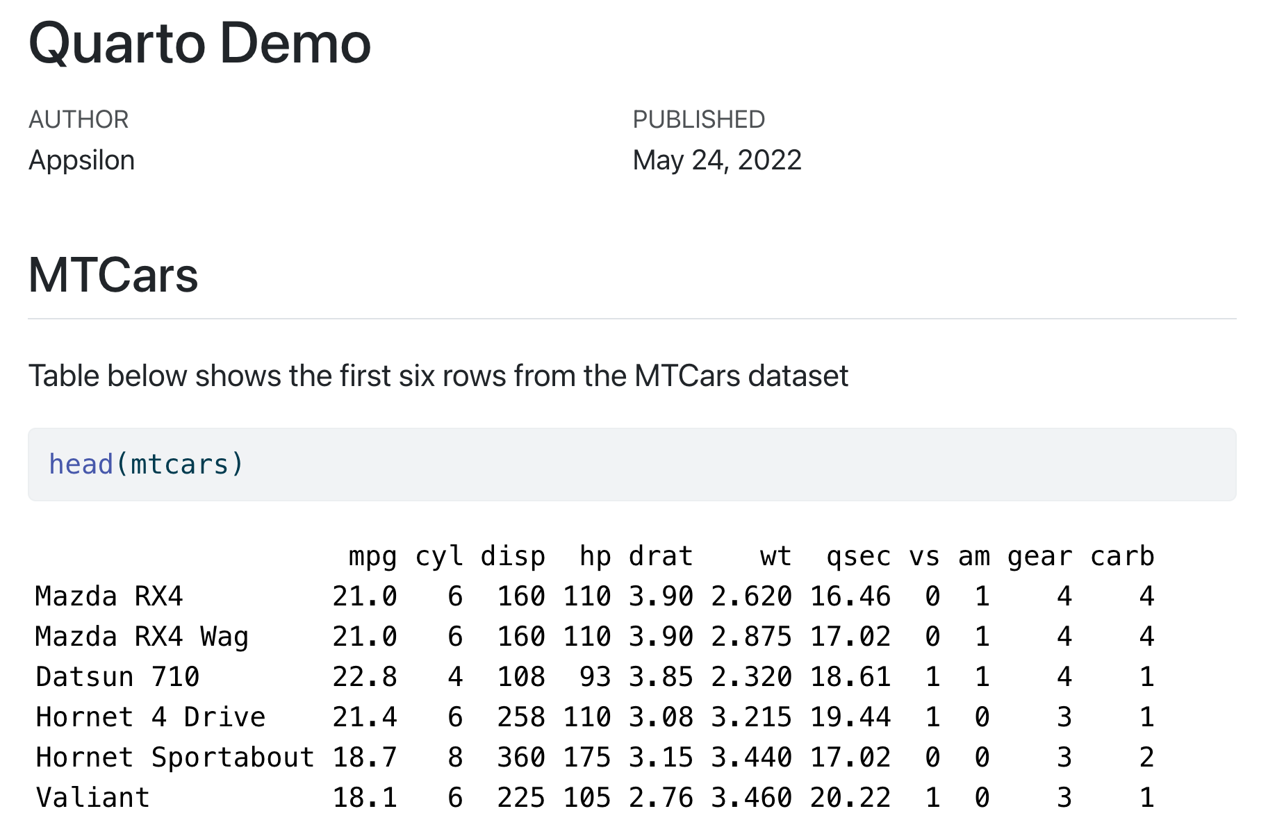
Image 5 – Rendered R Quarto document (2)

Amazing! Both code and table are rendered with beautiful stylings. If you hover over the code block, you’ll see an option to copy it with a single click. That feature is particularly useful for longer code snippets, and you don’t have to lift a finger to implement it.

Render Chart with Quarto

Let’s also see how to render a chart with Quarto. The procedure is identical – just add the code – but there are a couple of things you can tweak. First, it’s a good practice to reference a figure. In Quarto, that’s done by writing @figure-name in the text and then assigning labels to the figure in the code. The other good practice is to add a caption to your figures. Sure, you can add it directly through ggplot2, but adding it through Quarto will automatically match the text to document styles.

Long story short, here’s how to add a scatter plot to a Quarto document:

@fig-mtscatter shows a relationship between `wt` and `mpg` features in the MTCars dataset.
```{r}
#| label: fig-mtscatter
#| fig-cap: Weight of vehicle per 1000lbs (wt) vs. Miles/Gallon (mpg)

library(ggplot2)

ggplot(mtcars, aes(x = wt, y = mpg)) + 
    geom_point(color = "#0099f9", size = 5)
```

And here’s what it looks like when rendered:

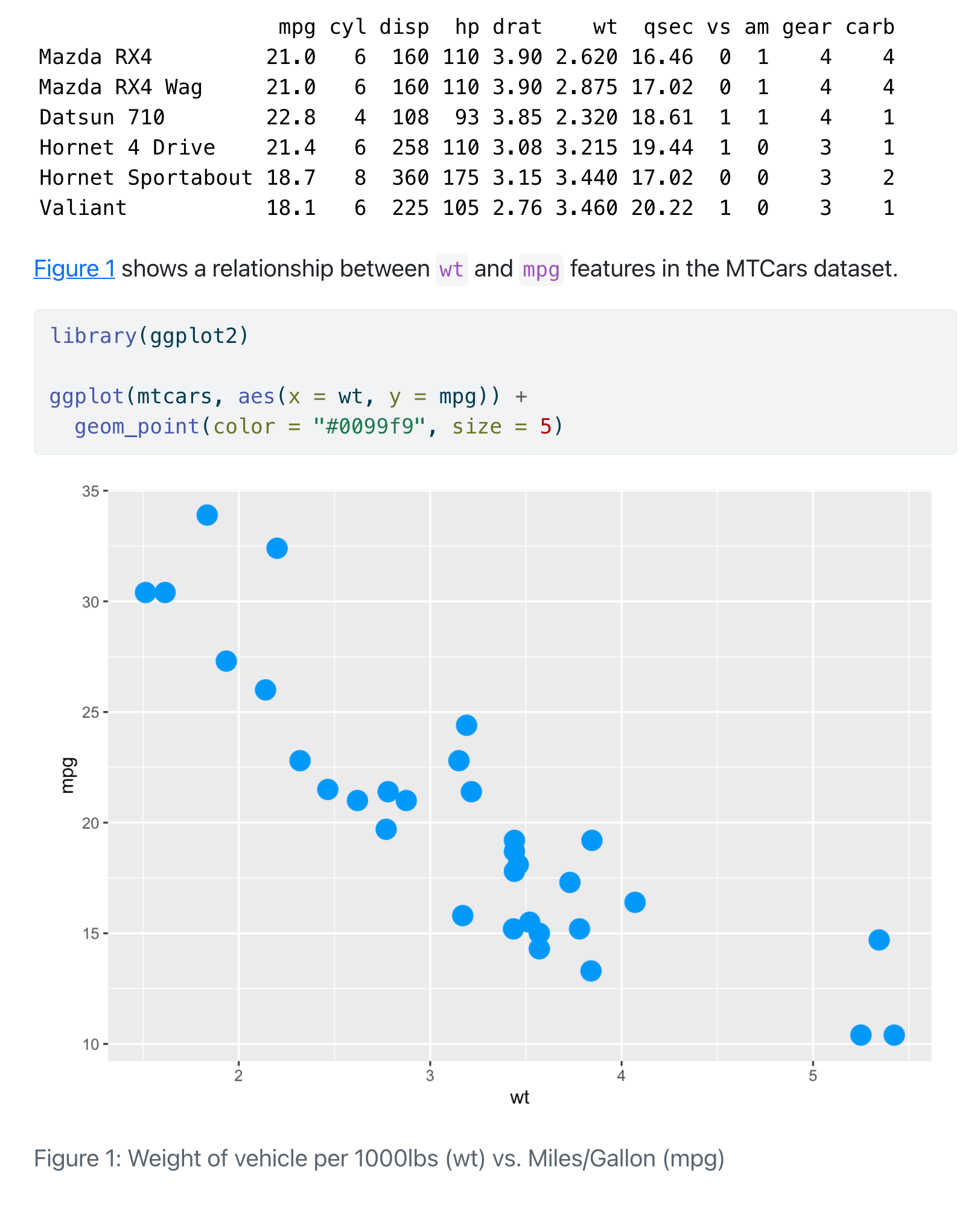
Image 6 – Rendered R Quarto document (3)

Are you new to data visualization in R? Here’s a complete guide to scatter plots.

And that’s how you can create a basic Quarto document! Next, let’s see how you can export it.

How to Export R Quarto Documents

There are numerous ways of exporting Quarto documents. Some options include HTML, ePub, Open Office, Web, Word, and PDF. We’ll show you have to work with the last two options, as these are the most common.

First, let’s address Microsoft Word. All you have to do is to add a couple of lines to the YAML header of the Markdown file. The example below shows how to add a table of contents with a custom title alongside some other options. Here’s a full reference manual, if you’re interested to learn more.

---
title: "Quarto Demo"
author: "Appsilon"
date: "2022-5-24"
format:
    docx:
        toc: true
        toc-depth: 2
        toc-title: Table of contents
        number-sections: true
        highlight-style: github
---

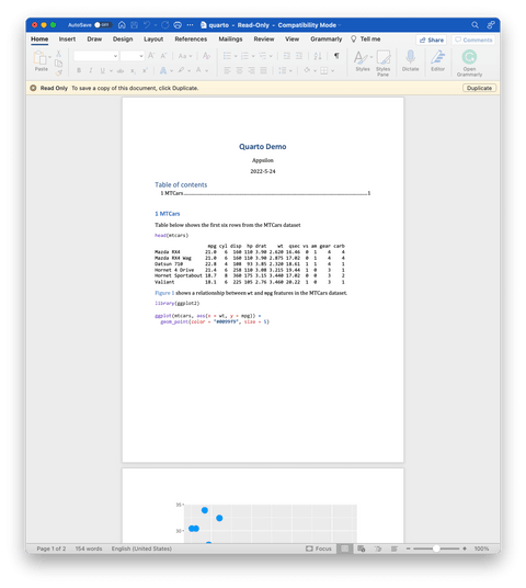
After rendering, the MS Word document will be opened automatically. It’s also saved to the same directory where your .qmd document is located. Here’s what it looks like on our end:

Image 7 – Rendered Word document

It’s read-only by default, but you can always duplicate it to make changes. Onto the PDF now. Before starting, you’ll need to install a distribution of TeX. TinyTeX is recommended by Quarto authors, so that’s what we’ll use. Run this line from the shell:

quarto tools install tinytex

Once installed, modify the YAML header accordingly. Here’s an entire formatting reference.

---
title: "Quarto Demo"
author: "Appsilon"
date: "2022-5-24"
format:
    pdf:
        toc: true
        toc-depth: 2
        toc-title: Table of contents
        number-sections: true
        highlight-style: github
---

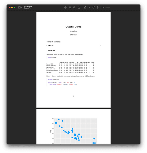
As you can see, the only change you had to do is to replace docx with pdf – all arguments are identical. Here’s what the document looks like:

Image 8 – Rendered PDF document

And that’s how you can export R Quarto Markdown files to Word and PDF documents. As mentioned, other options are available, but we won’t cover them today.

Summing up the R Quarto tutorial

Today you’ve learned the basics of creating highly-customizable Markdown documents in R Quarto. The package is a breeze to work with, and the documentation is easy to get around with.

If you’re developing packages for R, Python, or Julia, there’s no reason not to use Quarto to create amazing documentation around your product. It’s much more capable than other alternatives, and also has all the exporting options you’ll need.

Thinking about a career in R and R Shiny? Here’s everything you need to know to land your first job.

If you decide to give R Quarto a try, make sure to let us know. Share your Markdown documents with us on Twitter – @appsilon. We’d love to see what you come up with.