The standard procedure to create a Shiny app is straightforward. It involves a single app.R with a ui.R and server.R. But this simplicity also makes it difficult to build production-grade Shiny apps. At Appsilon, we have something different in our toolbox; we use Rhino.
TOC:
- What is Rhino?🦏
- Similar options to the Rhino R package🟰
- How to install Rhino⬇️
- How to use Rhino🧰
- Example Shiny build using Rhino🤷
- Let’s talk Modules and Rhino⚙️
- Managing Libraries with Rhino🔖
- Chart example 📈
- Table example 🔨
- Finishing touches: Logic🤖
- Finishing touches: Style🎨
- Complete Shiny app with Rhino🪄
What is Rhino anyway?🦏
Rhino is an opinionated framework focusing on best practices and development tools for R Shiny developers. The origins of the Rhino R package start from an internal need at Appsilon to avoid repetitive tasks, unify architecture, and codify our practices.
Rhino’s core benefits to our R/Shiny development process:
- Save time and avoid repetitive tasks by including best practices we value at the start of a project
- Unify applications’ architecture by providing sensible defaults.
- Automate and codify Appsilon practices to pass on knowledge in the form of code
Over the years, we took our collective experience across projects – noting challenges and what worked and didn’t work for us as a team. We built internal tools to address these issues and help structure our projects for faster, more successful outcomes.
Now that the Rhino project has evolved into an R package we are excited to share it with the Shiny community.
Please note that Rhino is in its early stages. We hope that by making the package public we can achieve two things. Firstly, share our knowledge base with the community and secondly, receive feedback from users. We invite you to test out Rhino and submit feedback.
Similar options to the Rhino R package🟰
Rhino was built with our enterprise dev needs in mind. But we believe ‘biodiversity’ is key for a healthy Shiny ecosystem. And that means one solution isn’t the right fit for every project.
There are other options from workflow packages to well-established toolkits. If you’re searching for the right solution, we encourage you to check out the options listed below.
The following mentions common solutions and how Rhino differs:
- golem: Rhino apps are not R packages. Rhino puts more emphasis on development tools, clean configuration, and minimal boilerplate and tries to provide default solutions for typical problems and questions in these areas.
- leprechaun: Leprechaun works by scaffolding Shiny apps, without adding dependencies. Rhino minimizes generated code and aims to provide a complete foundation for building Shiny apps ready for deployment in enterprise so that you can focus on the application’s logic and user experience.
- devtools: devtools streamlines package development. Rhino is a complete framework for building Shiny apps. Rhino features are interdependent (e.g. coverage and unit tests) and cannot be used without making the app into a basic Rhino structure.
- usethis: usethis adds independent code snippets you ask it to. Rhino is a complete framework for building Shiny apps. Your app is designed to call Rhino functions instead of having them insert code into your project.
Each of these has value, and depending on the project may be a more appropriate option. If you need assistance feel free to reach out to us to get your team on the right path.
How to install the Rhino package?⬇️
To install the Rhino package run:
install.packages(“rhino”)
How to use Rhino?🧰
Whether you are starting a new project or migrating an existing app – using Rhino is straightforward.
The simple-r method🤯
If you use RStudio, probably the easiest way to create a new Rhino application is to simply use the Create New Project feature. Once Rhino is installed, it will be automatically added as one of the options in RStudio.
Choose it, input the new project name, and you are ready to go.
The simple method🙂
To initialize a new Rhino project, run the init function:
rhino::init(“RhinoApplication”)
In running the app this way, Rhino will not change your working directory (wd). To do so, you will need to open a new R session in your new application directory or manually change the wd.
Example Shiny build using Rhino🤷
Now, we will build a simple app about… you guessed it: Rhinos! 🦏
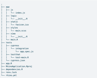
If everything is set up correctly, you will have the following files in your directory:
Running a Shiny application▶️
To run your newly minted Rhino application, you have to use the following command:
shiny::runApp()
It does not get simpler than this, does it? In any case, if you followed all the steps, you should be able to run the application successfully, and it should have the standard “Hello” message on the screen.
Let’s talk Modules and Rhino⚙️
Modules are R/Shiny’s way of keeping things simple, and Rhino capitalizes on that ability. In short, modules help you keep a logical division between different parts of the apps. For example, in an application that serves a map as well as a barplot, in most cases, it would make sense to have separate modules for both of these.
Also, since R/Shiny relies heavily on namespacing correctly, modules resolve this naturally and solve it without you worrying about it. We don’t have to dive deep into modules here, but if you are curious, here is more about it on the official RStudio Shiny Documentation.
In Rhino, each application view is intended to live as a Shiny module and use encapsulation provided by the {box} package.
{box}-ed in📦
The {box} library makes it incredibly easy to divide your code into logical modules. In other words, it enables modularization by giving you the ability to treat each kind of functionality in an isolated way. Imagine creating local libraries for your code that have functions your app needs. Now, imagine if the function is only used in two places instead of your entire app. In vanilla R/Shiny you would have to rely on loading the functions globally using something like a global.Rfile. {box} makes it possible for you to load the functions and variables only where you need them.
That is a lot of words to suggest something as follows. Let’s say we have a function that drills down into the sales data. Let’s assume it’s called drill_down_sales()and this function is exported using @export from a file called sales_utils.R. Now if we have two modules: plot and header, out of them, only plot seems to need this function.
We can then use box::use(sales_utils[drill_down_sales]) in the mod_plot.R file. The function will only be available to this file in question and it would make our imports simpler.
If you are familiar with Python, think about how we often use the from LIBRARY import FUNCTION. That is what {box} allows us to do.
Building our first Module🏗️
To begin, we will build our first module in the app/view/ directory. We can do that by using the following code block and for now, we don’t have to worry about actually building the chart:
# app/view/chart.R

box::use(
  shiny[h3, moduleServer, NS],
)

#' @export
ui <- function(id) {
  ns <- NS(id)

  h3("Chart")
}

#' @export
server <- function(id) {
  moduleServer(id, function(input, output, session) {
    print("Chart module server part works!")
  })
}
Look how it all comes together: the {box} usage, the R/Shiny moduleServer command, the NS() function to resolve the namespace.
Calling a Module📶
To call a module, we first need to import it into the main.R. How do we do that? Let’s use {box} once again:
# app/main.R

box::use(
  app/view/chart,
)

...
Once imported, the chart module will be ready for us in the main.R. We can then call each of its ui and server components using chart$ui() and chart$server(). They should work naturally since that is how everything is structured in Rhino and how it leverages {box}.
Let’s import things to the main.R, and call the functions from our chart module:
# app/main.R

box::use(
  shiny[bootstrapPage, moduleServer, NS],
)
box::use(
  app/view/chart,
)

#' @export
ui <- function(id) {
  ns <- NS(id)

  bootstrapPage(
    chart$ui(ns("chart"))
  )
}

#' @export
server <- function(id) {
  moduleServer(id, function(input, output, session) {
    chart$server("chart")
  })
}
Managing Libraries with Rhino🔖
Alright. So now we know how we can create modules and import them within the files of our Rhino project. But the power of programming is not in making everything yourself or reinventing the wheel, but rather using what is already made. What would an R project without {tidyverse} even look like!? In Rhino, we rely on the {renv} package to manage these dependencies, and we have a separate dependencies.R where we can simply define what we rely on.
To install a library, all you have to do is something like the following in the R Console:
# In R console
renv::install(c("dplyr", "echarts4r", "htmlwidgets", "reactable", "tidyr"))
Then, we simply need to import all these packages using the library() call in dependencies.R:
# dependencies.R

# This file allows packrat (used by rsconnect during deployment) to pick up dependencies.
library(dplyr)
library(echarts4r)
library(htmlwidgets)
library(reactable)
library(rhino)
library(tidyr)
But how do we make sure our packages are available when someone else uses the same project or when we deploy it on a server? We take a snapshot!
# in R console
renv::snapshot()
The renv::snapshot() command will simply pick up each of the packages imported in dependencies.R and create a renv.lock file. This file will have every package, along with the repository such as CRAN, MRAN, or others along with the version number and details for the library/package as well. Of course, you can also include local packages this way!
To add the dependencies to a module, you simply use the {box} package again.
# app/view/chart.R

box::use(
  echarts4r,
  shiny[h3, moduleServer, NS, tagList],
)

...
Let’s build a Chart!📈
Now that the chart.R is all ready, we can use the {echarts4r} import and develop the plot that we need to display.
# app/view/chart.R

box::use(
  echarts4r,
  shiny[h3, moduleServer, NS, tagList],
)

#' @export
ui <- function(id) {
  ns <- NS(id)

  tagList(
    h3("Chart"),
    echarts4r$echarts4rOutput(ns("chart"))
  )
}

#' @export
server <- function(id) {
  moduleServer(id, function(input, output, session) {
    output$chart <- echarts4r$renderEcharts4r( # Datasets are the only case when you need to use :: in `box`. # This issue should be solved in the next `box` release. rhino::rhinos |>
        echarts4r$group_by(Species) |>
        echarts4r$e_chart(x = Year) |>
        echarts4r$e_line(Population) |>
        echarts4r$e_x_axis(Year) |>
        echarts4r$e_tooltip()
    )
  })
}
The code above will simply use the dataset and plot the Rhino data as a line chart which would look something like the following:
Let’s build a Table!🔨
By now, we believe you have caught the gist of it. To create a table, we would go back to creating a new module. So, let us create app/view/table.R. Here is what you can use to build it.
# app/view/table.R

box::use(
  shiny[h3, moduleServer, NS, tagList],
)

#' @export
ui <- function(id) {
  ns <- NS(id)

  tagList(
    h3("Table")
  )
}

#' @export
server <- function(id) {
  moduleServer(id, function(input, output, session) {

  })
}
…and when you call it to the main.R, it would follow suit as well!
# app/main.R

box::use(
  shiny[bootstrapPage, moduleServer, NS],
)
box::use(
  app/view/chart,
  app/view/table,
)

#' @export
ui <- function(id) {
  ns <- NS(id)

  bootstrapPage(
    table$ui(ns("table")),
    chart$ui(ns("chart"))
  )
}

#' @export
server <- function(id) {
  moduleServer(id, function(input, output, session) {
    table$server("table")
    chart$server("chart")
  })
}
It’s getting simpler, isn’t it?
To Summarise: A new feature equals a new module that goes into app/view/. Each module then is imported into the main.R using {box} and once done, it can be used in the UI and server asmodule$ui() and module$server(). The amount of time this saves once set up correctly is wonderful. In fact, in more advanced usage, you can even call modules within modules and then call the parent module into the main. The possibilities are practically endless, and we expect you to go the extra mile in finding them!
Build a Table (for real this time)👀
In any case, for now, let’s update the table.R to actually build a table. For that, first, we will update the main.R.
# app/main.R

box::use(
  shiny[bootstrapPage, moduleServer, NS],
)
box::use(
  app/view/chart,
  app/view/table,
)

#' @export
ui <- function(id) {
  ns <- NS(id)

  bootstrapPage(
    table$ui(ns("table")),
    chart$ui(ns("chart"))
  )
}

#' @export
server <- function(id) {
  moduleServer(id, function(input, output, session) {
    # Datasets are the only case when you need to use :: in `box`.
    # This issue should be solved in the next `box` release.
    data <- rhino::rhinos

    table$server("table", data = data)
    chart$server("chart", data = data)
  })
}
We are now using the same dataset in the two modules. If you are feeling experimental, you can even have modules return values and then use them in the other modules. Rhino does not break the standard R/Shiny reactivity. In fact, it enhances it. All your modules can share resources, talk to each other and achieve cool things together!
Now, we update the table.R:
# app/view/table.R

box::use(
  shiny[h3, moduleServer, NS, tagList],
)

#' @export
ui <- function(id) {
  ns <- NS(id)

  tagList(
    h3("Table")
  )
}

#' @export
server <- function(id, data) {
  moduleServer(id, function(input, output, session) {

  })
}
…and also, the chart.R:
# app/view/chart.R

box::use(
  echarts4r,
  shiny[h3, moduleServer, NS, tagList],
)

#' @export
ui <- function(id) {
  ns <- NS(id)

  tagList(
    h3("Chart"),
    echarts4r$echarts4rOutput(ns("chart"))
  )
}

#' @export
server <- function(id, data) {
  moduleServer(id, function(input, output, session) {
    output$chart <- echarts4r$renderEcharts4r( data |>
        echarts4r$group_by(Species) |>
        echarts4r$e_chart(x = Year) |>
        echarts4r$e_line(Population) |>
        echarts4r$e_x_axis(Year) |>
        echarts4r$e_tooltip()
    )
  })
}
Since both modules now use the same data source, we can use the function parameter datato achieve our logic. Also, let’s now use {reactable} to finally build the table!:
# app/view/table.R

box::use(
  reactable,
  shiny[h3, moduleServer, NS, tagList],
)

#' @export
ui <- function(id) {
  ns <- NS(id)

  tagList(
    h3("Table"),
    reactable$reactableOutput(ns("table"))
  )
}

#' @export
server <- function(id, data) {
  moduleServer(id, function(input, output, session) {
    output$table <- reactable$renderReactable(
      reactable$reactable(data)
    )
  })
}
The app will start to look like this:
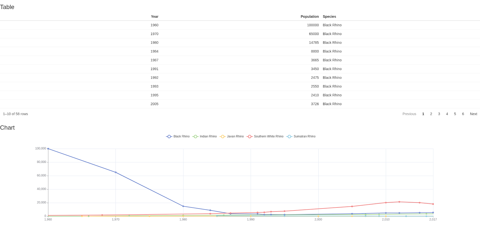
The cool thing here is that if you want to modify the plot, you now have a specific file (or module!) to go to, and if you want to move the table in a different way, you know you can go to its module. When you are inclined to change the overall layout or structure, you have the main.R to edit! Isn’t that simple? This is the power of Rhino!
Finishing touches: Shiny app Logic 🤖
Now that we are done with the core content of the app, it would make sense to add some interaction to it. That is where the logic side of things comes into play. Let’s try to transform the data a bit. Ideally, we want to show each species in a separate column to compare them properly in the table.
Let’s create a file called app/logic/data_transformation.R:
# app/logic/data_transformation.R

box::use(
  tidyr[pivot_wider],
)

#' @export
transform_data <- function(data) {
  pivot_wider(
    data = data,
    names_from = Species,
    values_from = Population
  )
}
Now, we need to call the function in the table module using the same box::use syntax we have been using so far.
# app/view/table.R

box::use(
  reactable,
  shiny[h3, moduleServer, NS, tagList],
)
box::use(
  app/logic/data_transformation[transform_data],
)

#' @export
ui <- function(id) {
  ns <- NS(id)

  tagList(
    h3("Table"),
    reactable$reactableOutput(ns("table"))
  )
}

#' @export
server <- function(id, data) {
  moduleServer(id, function(input, output, session) {
    output$table <- reactable$renderReactable( data |>
        transform_data() |>
        reactable$reactable()
    )
  })
}
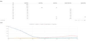
Once it’s done, you should now have a table that looks like the following:
Something seems off though. The table is arranged by the Black Rhino population. Ideally, it should be arranged by year. Let’s use {dplyr} for that and modify data_transformation.R:
# app/logic/data_transformation.R

box::use(
  dplyr[arrange],
  tidyr[pivot_wider],
)

#' @export
transform_data <- function(data) { pivot_wider( data = data, names_from = Species, values_from = Population ) |>
    arrange(Year)
}
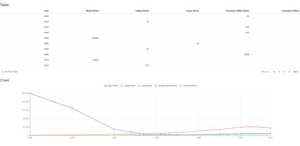
The result? A table that makes more sense in terms of information.
But there is still something off. The graph shows comma separators in the x-axis, which is actually a list of years. We do not use separators in these but in the R/Shiny world, nothing is impossible.
Let’s create a new file called app/logic/chart_utils.R:
# app/logic/chart_utils.R

box::use(
  htmlwidgets[JS],
)

#' @export
label_formatter <- JS("(value, index) => value")
Then, we add it to the chart module:
# app/view/chart.R

box::use(
  echarts4r,
  shiny[h3, moduleServer, NS, tagList],
)
box::use(
  app/logic/chart_utils[label_formatter],
)

#' @export
ui <- function(id) {
  ns <- NS(id)

  tagList(
    h3("Chart"),
    echarts4r$echarts4rOutput(ns("chart"))
  )
}

#' @export
server <- function(id, data) {
  moduleServer(id, function(input, output, session) {
    output$chart <- echarts4r$renderEcharts4r( data |>
        echarts4r$group_by(Species) |>
        echarts4r$e_chart(x = Year) |>
        echarts4r$e_line(Population) |>
        echarts4r$e_x_axis(
          Year,
          axisLabel = list(
            formatter = label_formatter
          )
        ) |>
        echarts4r$e_tooltip()
    )
  })
}
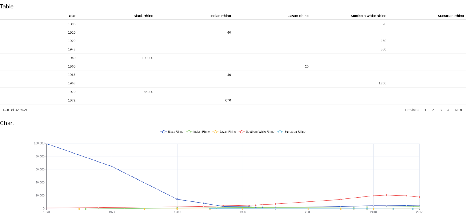
All in all, we have added a logic layer to our modules and both of them have received several improvements. Logic layers can be more extensive and detailed than just changing the format or adding some transformation. In fact, for more complex Shiny apps, Rhino makes it easier for you to integrate multiple pieces of logic into your modules with ease while keeping a logical separation between functions. For example, regardless of which module your functions are used in, all related functions remain in the same app/logic file. This makes it easier to maintain the code and make functions talk to each other.
Finishing touches: Shiny app Style🎨
Our app works but does it look great? Not yet. Right now it looks a bit barebones and we can change that easily! Rhino allows you to use sass using the {sass} package in R.
Adding some Sass💁
Note: The Rhino SASS builder uses Node.js. To run it without Node, you can change the sass label’s value from “node” to “r” in the rhino.yml file. This will make the builder leverage the R package for the SASS building. However, it uses a deprecated C++ library, so we feel the Node solution is the default and it is also our recommendation.
Rhino helpfully offers an app/styles directory to house all your SASS files as well as any partials you create. Where there is CSS (or SASS) there are classes and ids. Let’s add some to our project.
First, we will add a class “components-container” to the main.R file:
# app/main.R

box::use(
  shiny[bootstrapPage, div, moduleServer, NS],
)
box::use(
  app/view/chart,
  app/view/table,
)

#' @export
ui <- function(id) {
  ns <- NS(id)

  bootstrapPage(
    div(
      class = "components-container",
      table$ui(ns("table")),
      chart$ui(ns("chart"))
    )
  )
}

#' @export
server <- function(id) {
  moduleServer(id, function(input, output, session) {
    # Datasets are the only case when you need to use :: in `box`.
    # This issue should be solved in the next `box` release.
    data <- rhino::rhinos

    table$server("table", data = data)
    chart$server("chart", data = data)
  })
}
Now, we will add “component-box” to the chart.R file in app/view:
# app/view/chart.R

box::use(
  echarts4r,
  shiny[div, moduleServer, NS],
)
box::use(
  app/logic/chart_utils[label_formatter],
)

#' @export
ui <- function(id) {
  ns <- NS(id)

  div(
    class = "component-box",
    echarts4r$echarts4rOutput(ns("chart"))
  )
}

#' @export
server <- function(id, data) {
  moduleServer(id, function(input, output, session) {
    output$chart <- echarts4r$renderEcharts4r( data |>
        echarts4r$group_by(Species) |>
        echarts4r$e_chart(x = Year) |>
        echarts4r$e_line(Population) |>
        echarts4r$e_x_axis(
          Year,
          axisLabel = list(
            formatter = label_formatter
          )
        ) |>
        echarts4r$e_tooltip()
    )
  })
}
And now, the same class as above to the table.R file or the table module:
# app/view/table.R

box::use(
  reactable,
  shiny[div, moduleServer, NS],
)
box::use(
  app/logic/data_transformation[transform_data],
)

#' @export
ui <- function(id) {
  ns <- NS(id)

  div(
    class = "component-box",
    reactable$reactableOutput(ns("table"))
  )
}

#' @export
server <- function(id, data) {
  moduleServer(id, function(input, output, session) {
    output$table <- reactable$renderReactable( data |>
        transform_data() |>
        reactable$reactable()
    )
  })
}
Let’s write some CSS for the classes now. You can house the SASS or .scss files in app/styles/main.scss to begin with.
// app/styles/main.scss

.components-container {
  display: inline-grid;
  grid-template-columns: 1fr 1fr;
  width: 100%;

  .component-box {
    padding: 10px;
    margin: 10px;
    box-shadow: 0 4px 8px 0 rgba(0, 0, 0, 0.2), 0 6px 20px 0 rgba(0, 0, 0, 0.19);
  }
}
But if you try running the app after making the change above, you will notice nothing has changed. If you remember our Note from this section, this is where the building of SASS comes into play.
# in R console
rhino::build_sass()
It should now look something like the following:

Looks much neater, doesn’t it? We have the plots in separate boxes and they seem like they give different pieces of information about the same topic.
Let’s now add a title to the application by changing the main.R:
# app/main.R

box::use(
  shiny[bootstrapPage, div, h1, moduleServer, NS],
)
box::use(
  app/view/chart,
  app/view/table,
)

#' @export
ui <- function(id) {
  ns <- NS(id)

  bootstrapPage(
    h1("RhinoApplication"),
    div(
      class = "components-container",
      table$ui(ns("table")),
      chart$ui(ns("chart"))
    )
  )
}

...
And let’s add some styling again:
// app/styles/main.scss

.components-container {
  display: inline-grid;
  grid-template-columns: 1fr 1fr;
  width: 100%;

  .component-box {
    padding: 10px;
    margin: 10px;
    box-shadow: 0 4px 8px 0 rgba(0, 0, 0, 0.2), 0 6px 20px 0 rgba(0, 0, 0, 0.19);
  }
}

h1 {
  text-align: center;
  font-weight: 900;
}
Of course, we need to build the SASS again using build_sass():
# in R console
rhino::build_sass()

It is important to note that Rhino takes care of adding app/static/app.min.css to the application header so there is no need for you to do so.
Interaction with JS🚀
Note: Rhino requires Node.js for this as well. You can still use regular JavaScript code but please ensure you add it to the app/static/js file and not the www/ folder like you would for vanilla JS.
Let’s add a button:
# app/main.R

box::use(
  shiny[bootstrapPage, div, h1, icon, moduleServer, NS, tags],
)
box::use(
  app/view/chart,
  app/view/table,
)

#' @export
ui <- function(id) {
  ns <- NS(id)

  bootstrapPage(
    h1("RhinoApplication"),
    div(
      class = "components-container",
      table$ui(ns("table")),
      chart$ui(ns("chart"))
    ),
    tags$button(
      id = "help-button",
      icon("question")
    )
  )
}

...
Let’s style it using its id (help-button):
// app/styles/main.scss

.components-container {
  display: inline-grid;
  grid-template-columns: 1fr 1fr;
  width: 100%;

  .component-box {
    padding: 10px;
    margin: 10px;
    box-shadow: 0 4px 8px 0 rgba(0, 0, 0, 0.2), 0 6px 20px 0 rgba(0, 0, 0, 0.19);
  }
}

h1 {
  text-align: center;
  font-weight: 900;
}

#help-button {
  position: fixed;
  top: 0;
  right: 0;
  margin: 10px;
}
Pro Tip: You need to build_sass() after every change to the SASS files. But there is another trick. If you create a new terminal, you can start an R instance in it and call rhino::build_sass() in watch mode using rhino::build_sass(watch = TRUE). As long as the terminal is active, it will continue to watch for changes in the SASS files (on every save).
In any case, once you add the styling to the button and build_sass(), it should show up on the app as it does in the screenshot below:

Let’s write the JS code to show a popup alert:
// app/js/index.js

export function showHelp() {
  alert('Learn more about Rhino: https://appsilon.github.io/rhino/');
}
If you’re familiar with JS, you may have noticed “export” being used before the function. In Rhino, you can write as many JS functions as you want, but only those with the keyword at the beginning will be available for the app. This extends the flexibility by you being able to experiment, only use certain functions, and try different approaches!
Now, just like with styles, you need to build the JS using rhino::build_js()
🥸Psst, the Pro-tip about the watch mode applies here, too.
By building both SASS and JS, we are essentially creating the app.min.css and app.min.js files which are minified versions of all the available styles and interaction code respectively. Both of these are automatically added to the <head> tag and you do not need to call them explicitly.
Let’s now call the function showHelp() in the main.R file:
# app/main.R

box::use(
  shiny[bootstrapPage, div, h1, icon, moduleServer, NS, tags],
)
box::use(
  app/view/chart,
  app/view/table,
)

#' @export
ui <- function(id) {
  ns <- NS(id)

  bootstrapPage(
    h1("RhinoApplication"),
    div(
      class = "components-container",
      table$ui(ns("table")),
      chart$ui(ns("chart"))
    ),
    tags$button(
      id = "help-button",
      icon("question"),
      onclick = "App.showHelp()"
    )
  )
}

...
Where did the “App” come from in App.showHelp()? This is the second important difference between making apps in Rhino. All your JS functions, regardless of which file they are in, if exported and included in app.min.js will be available in App, such as Math.round or any other JS library you know of. Makes things easier, right?
Running the application and clicking on the ❓button takes you here.
Complete Shiny app with Rhino🪄
Your Rhino app is now functional, styled, and ready for the world! This was a heavy tutorial with a lot of information in it so let’s recap a few key points.
- Rhino makes it easier to build an R/Shiny app by managing the app in
app/views, which are modules, split logically based on the functionality of the app. - All the packages, as well as local functions, are imported using
box::use(). - On the topic of local functions, all the logic you write goes to
app/logic. - To style things and add interaction, you can use SASS and JS. These can be created in
app/stylesandapp/js. - Both of them require Node. For SASS, if you do not have Node, you can use the r package by changing the
rhino.ymlfile’ssasslisting fromnodetor. - Both need their partner
build_*()functionsbuild_sass()andbuild_js()to condense them into theapp.min.cssandapp.min.jsfiles.
- Both of them require Node. For SASS, if you do not have Node, you can use the r package by changing the
- You can also use
watch = TRUEin thebuild_*()function calls in a new terminal to start a watch mode for them to avoid calling the function after every minor change.
- You can also use
And that’s it! These are all the things you need to remember to begin working on your Rhino application. It’s a lot to jump right in, but if you forget anything, feel free to explore the Rhino documentation. And if you need assistance with your enterprise project, reach out to our team for help!
Oh, and also, don’t forget to have fun! 👋
