


 Share
Share Tweet
Tweet Share
Share


![Semantic segmentation [left] and instance segmentation [right] (Image credit: www.analyticsvidhya.com).](/_gatsby/image/2e2ab18788251adef3e203ea8ea54008/37db8396691405347df1ca1002ab9cda/semantic-vs-instance-segmentation-in-ai.png?u=https%3A%2F%2Fwordpress.appsilon.com%2Fwp-content%2Fuploads%2F2021%2F10%2Fsemantic-vs-instance-segmentation-in-ai.png&a=w%3D316%26h%3D96%26fm%3Dpng%26q%3D90&cd=2023-03-07T11%3A41%3A47)


Unraveling the Segment Anything Model (SAM)

20 October 2023
Join the Shiny Community every month at Shiny Gatherings
This is the first blog of a three-part miniseries on developing an AI to detect solar panels from orthophotos. The articles will be broken down into three project steps:
fastaistreamlitBut before we jump into the project, we need to understand some of the basics.
The solar panel industry is booming. In 2020, the solar industry generated roughly $25 billion in private funding in the U.S. alone. With more than 10,000 solar companies across the U.S., a nearly 70% decline in installation costs, and competitive utility prices it’s no wonder 43% of new electric capacity additions to the American electrical grid have come from solar. Although it only makes up a meager 4% of all U.S. electricity production, the solar industry is seeing clear skies.
So how do economists and policymakers track this growth? Where should solar business owners target new markets? Is it even possible to monitor this adoption on such a massive scale? The answer to these questions and more lies in AI.
Because in an age when fossil fuels are beginning to darken our days, renewable sources of energy are starting to shine. From geothermal and wind turbines to hydropower and solar, our options are steadily improving. And with declining costs in technologies, adoption has been skyrocketing. But there are still improvements that can be made. Using AI and machine learning we can speed up adoption, improve sales, and track large-scale implementation.
So how do we hope to achieve this? By using AI to detect solar panels from satellite and aerial images!
AI is being used to increase response times to natural disasters and improve humitarian aid. Test Appsilon’s AI model for assessing building damage.
Open your google maps, zoom to a city, and turn on the satellite view. Chances are, you’re looking at one or two orthophotos. These are typically satellite images but can be aerial photographs from something like a plane or UAV. However, when you take an unprocessed image its features are likely distorted unless viewing from directly above the target area (aka “nadir”). Tall buildings, mountains, basically anything with elevation, will look like they’re leaning and straight lines like pipelines will “bend” with the topography.
Aerial photograph vs orthoimage showcasing distortion effects of terrain relief on a pipeline (Image from USGS, public domain).
In order to correct the parallax displacement from camera tilt and relief, we need to orthorectify the image, i.e. create a mathematical interpolation of the image using ground control points. This allows us to minimize the scale-warping effect as we move away from nadir. In doing so, we’ve created a photo with a uniform scale that can overlap other maps with minimal spatial errors.
Are you using AI for a social good project? Appsilon’s data science team can help through our Data4Good initiative.
But why is this important to identifying Solar Panels? Well, because regular satellite images don’t have a uniform scale, any attempts to quantify precise distances and areas would be inaccurate. For example, if you’re training a model to identify 1 x 1-meter solar panels on a hillside and calculate the total area, the farther away from nadir it goes, the more likely the panels are to distort in size. Your image segmentation and classification will probably be incorrect and your area measurements inaccurate.
If you’d like to follow along and create a model of your own, you can find open-source orthophotos in many places including ESRI’s orthophoto Basemaps and Poland’s Geoportal for orthomaps.
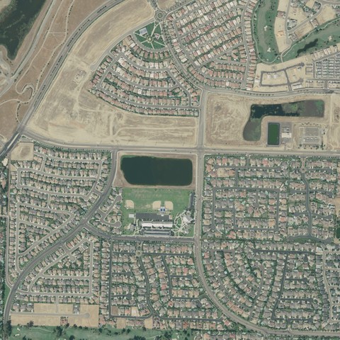
You can access the data we’ll be using to train our model from Distributed Solar Photovoltaic Array Location and Extent Data Set for Remote Sensing Object Identification. The dataset consists of 526 images of 5000 x 5000 px and 75 images at 6000 x 4000 covering four areas of California. The dataset also contains CSV files describing the locations of roughly 20,000 solar panels.
Aerial photograph of Californian suburbs. AI can find solar panels. Can you?
Once you have your images, you can think about the panel identification task as an image segmentation problem. To solve the problem, you’ll need to predict a class for each pixel of an image. In our case, we’ll keep it simple with two classes, “solar panel” and “not a solar panel.” So, we’ll try and predict whether a specific pixel belongs either to a solar panel or not.
To do this, we will first prepare training data, i.e. create an image segmentation mask. A segmentation mask is an image with the same bounds as the original image, but with information on the contents at the pixel level with a unique color for each class. This helps parse the image into important areas to focus on rather than processing the image as a whole.
There are two types of segmentation: semantic and instance. Semantic segmentation groups pixels of a similar class and assigns the same value to all in that group (e.g., people vs background seen in the image below). In our case, we’ll be creating semantic segmentation. If you’re looking to perform additional tasks like assigning subclasses or counting classes, you’ll want to create an instance segmentation mask.
Semantic segmentation [left] and instance segmentation [right] (Image credit: www.analyticsvidhya.com).
To build the model yourself, you’ll need to import a few libraries and load the necessary data. I’ll show you how, below:
from glob import glob
from pathlib import Path
from typing import List, Tuple

import numpy as np
import pandas as pd
from PIL import Image, ImageDraw
from tqdm.contrib.concurrent import process_map

root = Path('.')
df1 = pd.read_csv(root / 'polygonDataExceptVertices.csv')
df2 = pd.read_csv(root / 'polygonVertices_PixelCoordinates.csv')

df1.set_index('polygon_id', inplace=True)
df2.set_index('polygon_id', inplace=True)
all_images = df1['image_name'].unique()
As we will discover later,polygon_idis a unique column that serves as an ID. We should immediately set it as a pandas index. We can also explore a few columns from thepolygonDataExceptVertices.csvandpolygonVertices_PixelCoordinates.csvfiles.
df1.loc[:, ['image_name', 'city']]
df2.iloc[:, :8]
The first file details the folder structure and geospatial data related to the polygons of individual solar panel islands.
| polygon_id | image-name | city | |
| 0 | 1 | 11ska460890 | Fresno |
| 1 | 2 | 11ska460890 | Fresno |
| 2 | 3 | 11ska460890 | Fresno |
| 3 | 4 | 11ska460890 | Fresno |
| 4 | 5 | 11ska460890 | Fresno |
Each row in the second file describes a single polygon with the coordinates of its vertices.
| polygon_id | number_vertices | lon1 | lat1 | lon2 | lat2 | lon3 | lat3 | |
| 0 | 1 | 8 | 3360.5 | 131.631 | 3249.2 | 87.9851 | 3213.75 | 73.85 |
| 1 | 2 | 9 | 3361.15 | 69.6154 | 3217.62 | 12.8462 | 3217.44 | 13.0961 |
| 2 | 3 | 11 | 3358.02 | 48.1369 | 3358.05 | 48.15 | 3360.74 | 42.3793 |
| 3 | 4 | 9 | 2571.59 | 2068.05 | 2571.02 | 2067.39 | 2571.35 | 2067.15 |
| 4 | 5 | 9 | 2563.78 | 2091.4 | 2504.42 | 2021.67 | 2503.98 | 2022.05 |
To create segmentation masks we will process every image separately. Then for each image, we will locate and draw all polygons. We will use ImageDraw the PIL package to easily draw polygons on the images. Image.new("L", size) allows us to create a new image with one channel – black/white as this is what we need for the segmentation mask. We fill polygons with value 1 as the fastai library expects each class to have a sequential class number.
Since there are over 40GB of image files to process, it will take some time. Because every image can be processed simultaneously, we can easily parallelize calculations. Parallel map functionality with a progress bar is provided by the tqdm package, that’s what process_map function does. The process_map function requires a single argument so we have to wrap process_image as the function wrap_process_image does. Line 26 in process_all_images converts a list of lists into a unified list. Since image_data is a list of lists of tuples of the same length, it is easily convertible to pandas dataframe.
def process_image(img_name: str, rawimg_dir: Path, lab_dir: Path, img_dir: Path, out_s: int) -> List[Tuple]:
    intr_polys = df1.query("image_name == @img_name")
    im0 = Image.open(rawimg_dir / (img_name + ".tif"))
    ims = Image.new("L", im0.size)
    draw = ImageDraw.Draw(ims)
    for polyid, row in df2.iterrows():
        n_vert = int(row["number_vertices"])
        poly_verts = row[1:(1 + 2 * n_vert)]
        # a tricky way to obtain list of tuples of [(x[0], x[1]), (x[2], x[3]), ...]
        points = list(zip(poly_verts[::2], poly_verts[1::2]))
        if len(points) == 0:  # in case of missing values
            print(f"Polyid: {polyid} has no points")
            continue
        draw.polygon(points, fill=1)  # fill polygon with ones
    k1 = im0.size[0] // out_s
    k2 = im0.size[1] // out_s
    split_save_image(im0, img_name, img_dir, k1, k2)
    l = split_save_image(ims, img_name, lab_dir, k1, k2, True)
    return l

def wrap_process_image(img_name: str) -> List[Tuple]:
    return process_image(img_name, root/"raw_images", root/"labels", root/"images", 500)

def proccess_all_images(all_images: List[str], max_workers: int) -> pd.DataFrame:
    images_data: List[List[Tuple]] = process_map(wrap_process_image, all_images, max_workers=max_workers)
    return pd.DataFrame([ff for l in images_data for ff in l], columns=["file", "fill"])

max_workers = 4
res = proccess_all_images(all_images, max_workers)
The last missing piece is the split_save_image function. Original images of size 5000x5000px or 6000x4000px are far too big to process in a neural network. We have to split them into smaller pieces. That what split_save_image is for.
def split_save_image(im: Image, root:str, dir: Path, k1: int, k2: int, meta: bool = False) -> List[Tuple]:
    h, w = im.size
    dh = h / k1
    dw = w / k2

    l: List[Tuple] = []
    for i in range(k1):
        for j in range(k2):
            imc = im.crop((i*dh, j*dw, (i+1)*dh, (j+1)*dw))
            fname = dir/(f"root_{i}_{j}.png")
            imc.save(fname)
            if meta:
                nz_ratio = np.asarray(imc).sum() / (dh * dw)
                l.append((fname, nz_ratio))
    return l
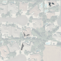
Here we decided to split images into 500 x 500 px patches. Because every image is split into 100 or 96 patches, many won’t contain solar panel fragments. But we won’t toss these out. At least not yet, because the images that are empty might prove to be useful later. If we pass the argument meta=True then after saving the image, the percentage of pixels occupied by solar panels will be calculated and added to the list. The example patch has been presented above.
Through Data4Good, Appsilon helps build support systems for disaster risk management in Madagascar.
The script will run for a while and process every image in the raw_images directory. It might take about 20 minutes. The progress bar will help to track the remaining time. The last thing to do is to save the data frame with a pixel-fill ratio.
res.to_csv("fill_ratio.csv", index=False)
res.head()
Now we end up with 59800, 500 x 500 px patches, and corresponding segmentation masks. Finally, we can visualize a sample patch and corresponding mask:
A mask containing polygons of solar panels.
To recap, in the first of this series, we downloaded orthophotos of solar panels in California and processed them by creating corresponding segmentation masks. Later we split images into smaller pieces to make them consumable for a neural network.
In part two we will use the fastai library to train a PoC model for solar panel detection.
Stay tuned!
Use Shiny to build elegant, engaging apps to better serve at-risk communities. Explore the possibilities of Shiny with Appsilon’s VisuaRISK application.

