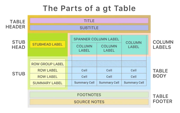
{gt} is an R package for displaying tables. Designed to bridge the gap between data analysis and publication-quality output, it is perfect for generating clinical tables ready for publication.
{gt} introduces a comprehensive, intuitive syntax for table creation, allowing users to craft detailed, aesthetically pleasing tables. It divides table components into the table header, the stub, the column and spanner column labels, the table body, and the table footer. This makes it extremely easy to format the output.
To discover packages used in clinical trial data analysis, check out our blog post: R Programming and Pharmaceutical Data Analysis (Packages for Clinical Trial Data).
Table of Contents
- Exploring Clinical Tables with gt
- Demographics and Baseline Characteristics Table
- Adverse Events Table
- Demographics and Baseline Characteristics Clinical Table with {gt}
- Adverse Events Clinical Table with {gt}
- Summing up Clinical Tables with {gt}
Exploring Clinical Tables with gt
{chevron} package documentation provides an immense catalogue of standard clinical tables. While numerous formats exist, we will concentrate on two primary types: the Demographics and Baseline Characteristics Table and the Adverse Events Table.
Demographics and Baseline Characteristics Table
This table format is crucial for displaying key demographic and baseline characteristics of study participants. It typically includes age, sex, race, and other relevant baseline information that can influence the outcome of the study.
By presenting this data, researchers can ensure that the study population is well-defined and that findings apply to the intended patient groups. It also aids in identifying any imbalances between treatment groups that could affect the results.
Adverse Events Table
The Adverse Events Table is essential for reporting any negative outcomes experienced by participants during the study. It groups adverse events into categories based on the body system affected. This grouping helps in the systematic presentation of adverse events, making it easier for readers to assess the safety profile of a drug or intervention.
Let’s create those clinical tables using the {gt} package!
Demographics and Baseline Characteristics Clinical Table with {gt}
For creating a demographic table, we will use the admiral_adsl example data frame from the {admiral} package.
library(admiral)
library(dplyr)
library(tidyr)
library(purrr)
library(gt) #Version: 0.10.1

admiral_adsl
#> # A tibble: 306 × 50
#> STUDYID USUBJID SUBJID RFSTDTC RFENDTC RFXSTDTC RFXENDTC RFICDTC RFPENDTC
#>
#> 1 CDISCPILOT… 01-701… 1015 2014-0… 2014-0… 2014-01… 2014-07… 2014-07…
#> 2 CDISCPILOT… 01-701… 1023 2012-0… 2012-0… 2012-08… 2012-09… 2013-02…
#> 3 CDISCPILOT… 01-701… 1028 2013-0… 2014-0… 2013-07… 2014-01… 2014-01…
#> 4 CDISCPILOT… 01-701… 1033 2014-0… 2014-0… 2014-03… 2014-03… 2014-09…
#> 5 CDISCPILOT… 01-701… 1034 2014-0… 2014-1… 2014-07… 2014-12… 2014-12…
#> 6 CDISCPILOT… 01-701… 1047 2013-0… 2013-0… 2013-02… 2013-03… 2013-07…
#> 7 CDISCPILOT… 01-701… 1057 2013-12…
#> 8 CDISCPILOT… 01-701… 1097 2014-0… 2014-0… 2014-01… 2014-07… 2014-07…
#> 9 CDISCPILOT… 01-701… 1111 2012-0… 2012-0… 2012-09… 2012-09… 2013-02…
#> 10 CDISCPILOT… 01-701… 1115 2012-1… 2013-0… 2012-11… 2013-01… 2013-05…
#> # ℹ 296 more rows
#> # ℹ 41 more variables: DTHDTC , DTHFL , SITEID , AGE ,
#> # AGEU , SEX , RACE , ETHNIC , ARMCD , ARM ,
#> # ACTARMCD , ACTARM , COUNTRY , DMDTC , DMDY ,
#> # TRT01P , TRT01A , TRTSDTM , TRTSTMF , TRTEDTM ,
#> # TRTETMF , TRTSDT , TRTEDT , TRTDURD , SCRFDT ,
#> # EOSDT , EOSSTT , FRVDT , RANDDT , DTHDT , …
Let’s clean the data by only including randomized subjects who have taken at least one dose of study medication according to the SAFFL (Safety Population Flag) and improve readability on the SEX and ETHNIC columns. We will also save treatments in the dataset.
safety_subjects <- admiral_adsl |>
  filter(SAFFL == "Y") |>
  mutate(
    SEX = case_when(
      SEX == "F" ~ "Female",
      SEX == "M" ~ "Male"
    ),
    ETHNIC = stringr::str_to_sentence(ETHNIC)
  )


treatments <- unique(safety_subjects$ACTARM)
The first step of creating any {gt} table is to summarize the data frame. The goal is to create a data frame such that every row represents a row in the final output, and each column helps us to group, format, or merge information.
In a demographic table, each row is a statistic (rowname_col argument in gt::gt) related to a demographic group (groupname_col argument in gt::gt) across treatments. For each of those rows, we have the value for the statistic and for some of them, we also have helper values that will be displayed alongside the actual value such as percentages and standard deviations.
Let’s create two functions for summarising numerical and categorical data in our data. Notice that in both functions, we create separate columns for the helper values we are going to merge with cols_merge.
categorical_summary <- function(categorical_column_name, groupname) { safety_subjects |>
    count(ACTARM, .data[[categorical_column_name]], name = "value") |>
    group_by(ACTARM) |>
    mutate(pct = value / sum(value)) |>
    pivot_wider(names_from = ACTARM, values_from = c(value, pct)) |>
    rename(rowname = all_of(categorical_column_name)) |>
    mutate(groupname = paste0(groupname, ", n (%)"))
}

numerical_summary <- function(numerical_column_name, groupname) {
  summary_stats <- safety_subjects |>
    group_by(ACTARM) |>
    summarise(
      n = n(),
      `Mean (SD)` = mean(.data[[numerical_column_name]]),
      Median = median(.data[[numerical_column_name]]),
      `Min - Max` = NA
    ) |>
    pivot_longer(n:`Min - Max`, names_to = "rowname", values_to = "value") |>
    pivot_wider(names_from = ACTARM, values_from = value, names_prefix = "value_") # nolint

  column_min_max <- safety_subjects |>
    group_by(ACTARM) |>
    summarise(
      min = min(.data[[numerical_column_name]]),
      max = max(.data[[numerical_column_name]])
    ) |>
    mutate(rowname = "Min - Max") |>
    pivot_wider(names_from = ACTARM, values_from = c(min, max))

  column_sd <- safety_subjects |>
    group_by(ACTARM) |>
    summarise(
      sd = sd(.data[[numerical_column_name]])
    ) |>
    mutate(rowname = "Mean (SD)") |>
    pivot_wider(names_from = ACTARM, values_from = sd, names_prefix = "sd_")

  summary_stats |>
    left_join(column_sd, by = "rowname") |>
    left_join(column_min_max, by = "rowname") |>
    mutate(groupname = groupname)
}
Now we can create the initial table with gt() function.
gt_data <- categorical_summary("SEX", "Sex") |>
  bind_rows(
    categorical_summary("AGEGR1", "Age Group"),
    categorical_summary("RACEGR1", "Race"),
    categorical_summary("ETHNIC", "Ethnicity"),
    numerical_summary("AGE", "Age (Years)")
  )

initial_table <- gt_data |>
  gt(
    rowname_col = "rowname",
    groupname_col = "groupname"
  )
initial_table
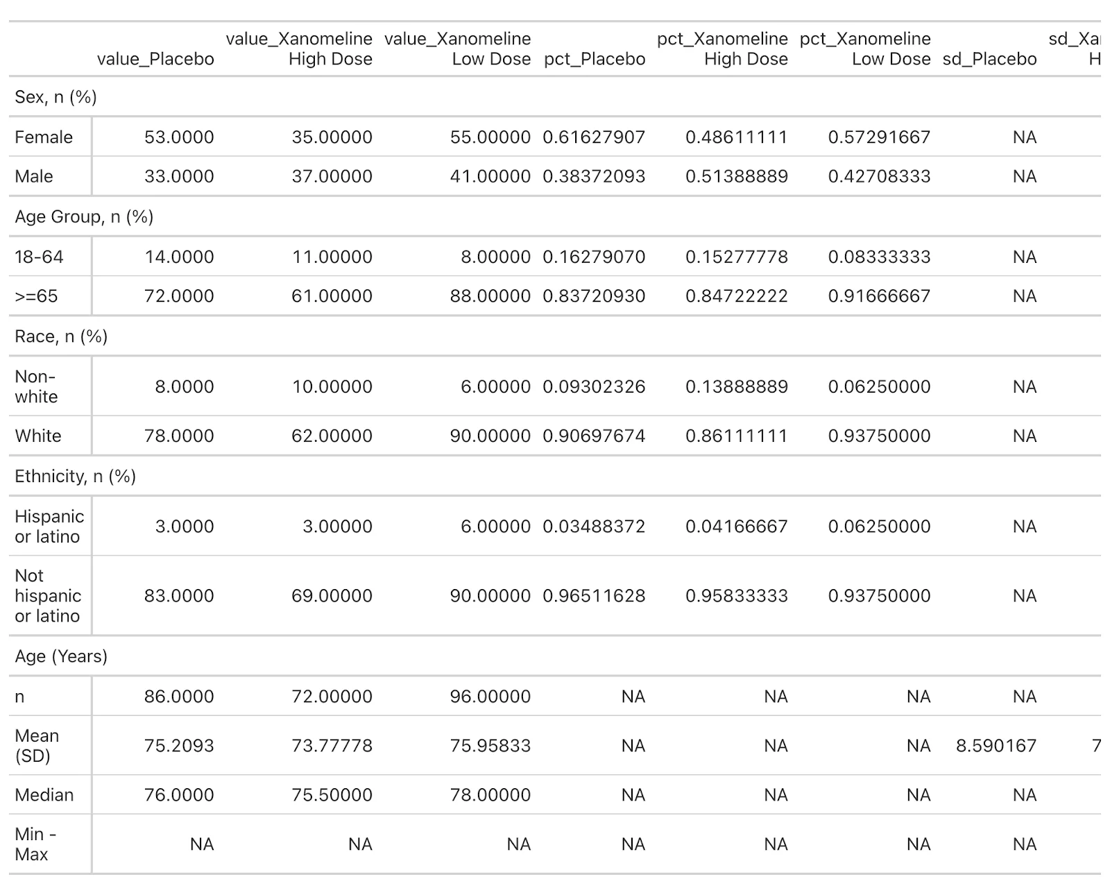
Demographic Distribution in Xanomeline Clinical Trial
Before merging any columns, we first format the individual columns/rows with the fmt_* functions.
formatted_table <- initial_table |>
  fmt_percent(
    columns = starts_with("pct_")
  ) |>
  fmt_integer(
    columns = starts_with("min_")
  ) |>
  fmt_integer(
    rows = all_of(c("n", "Median"))
  ) |>
  fmt_integer(
    columns = starts_with("value_"),
    rows = groupname == "Sex, n (%)"
  ) |>
  fmt_number(
    rows = "Mean (SD)",
    columns = starts_with("value_"),
    decimals = 1
  ) |>
  fmt_number(
    columns = starts_with("sd_")
  )
formatted_table
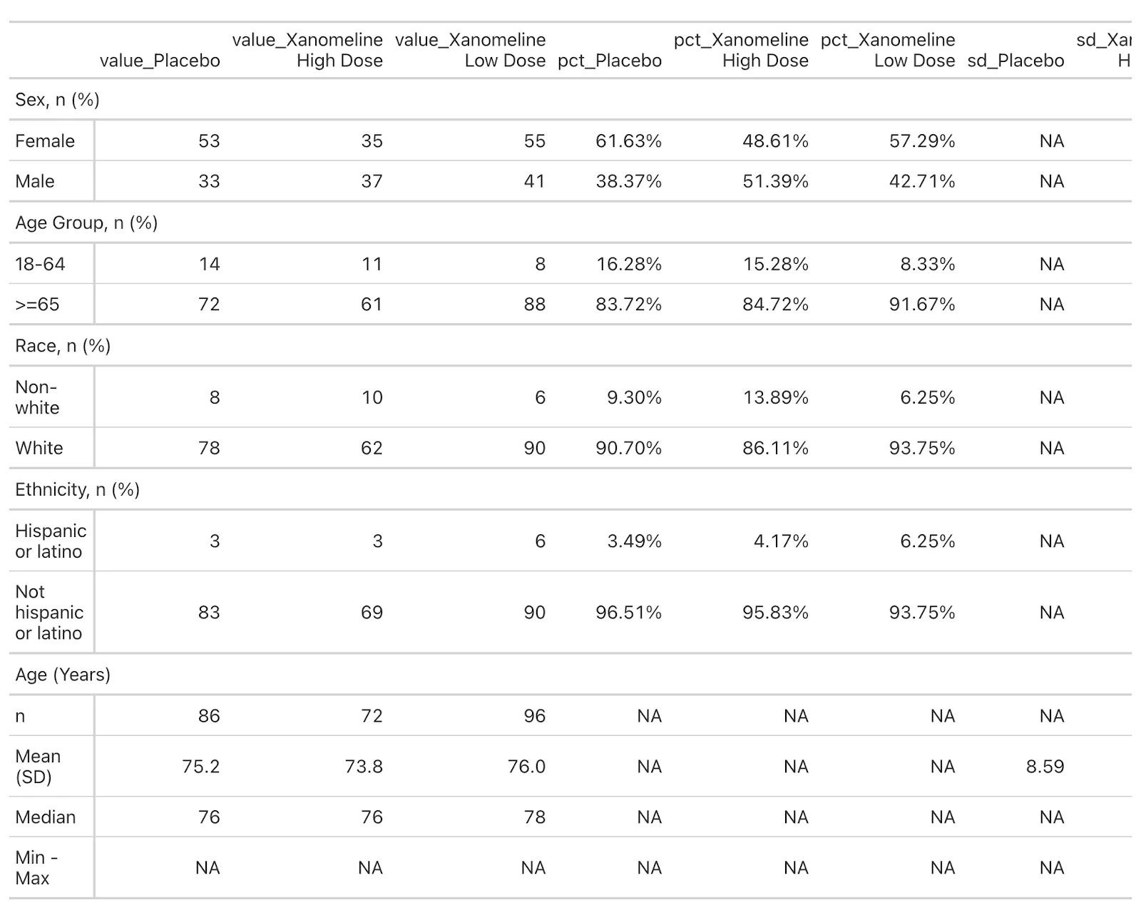
Demographic Data of Xanomeline Clinical Trial Participants
We can now proceed to merge columns for each treatment. cols_merge_n_pct handles NA values in col_pct automatically by omitting them. To avoid replicating the same code for each treatment, we will use purrr::reduce.
merged_table <- append(list(formatted_table), treatments) |>
  reduce(
    \(x, treatment) {
      x |>
        cols_merge_n_pct(
          col_n = paste0("value_", treatment),
          col_pct = paste0("pct_", treatment),
          rows = groupname %in% paste0(c("Sex", "Age Group", "Race", "Ethnicity"), ", n (%)")
        )
    }
  ) |>
  list() |>
  append(treatments) |>
  reduce(
    \(x, treatment) {
      x |>
        cols_merge(
          rows = "Min - Max",
          columns = c(
            paste0("value_", treatment), paste0("min_", treatment), paste0("max_", treatment)
          ),
          pattern = "{2} - {3}"
        )
    }
  ) |>
  list() |>
  append(treatments) |>
  reduce(
    \(x, treatment) {
      x |>
        cols_merge(
          columns = c(paste0("value_", treatment), paste0("sd_", treatment)),
          pattern = "{1} ({2})",
          rows = "Mean (SD)"
        )
    }
  )
merged_table
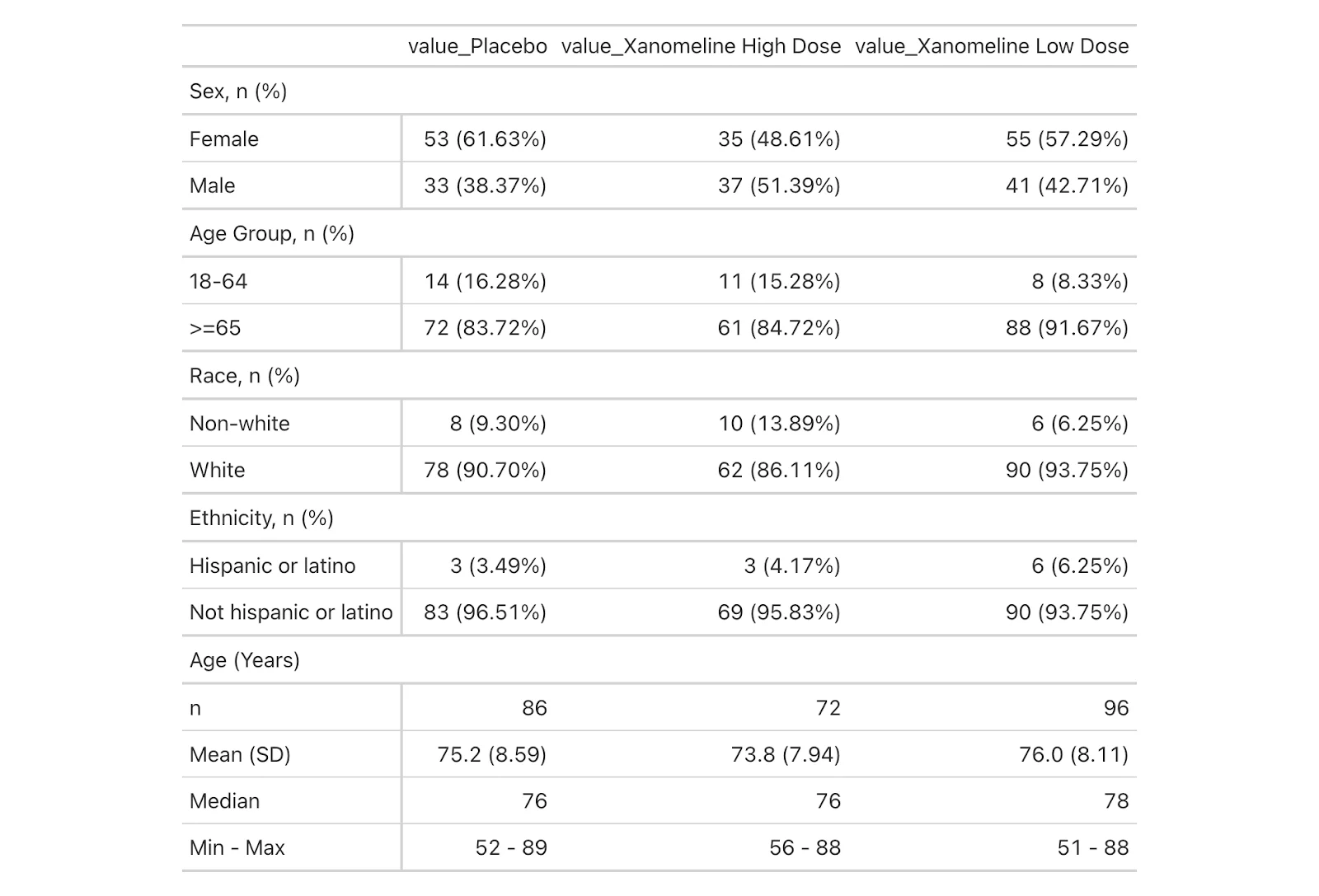
Clinical Trial Demographic Data Comparison
Now, we have a table that has the expected rows and columns; all we have to do is add the title and some styling. 🎨
column_labels <- safety_subjects |>
  count(ACTARM) |>
  mutate(
    label = paste0(ACTARM, " (N = ", n, ")"),
    gt_column_name = paste0("value_", ACTARM)
  )

column_labels <- setNames(column_labels$label, column_labels$gt_column_name) merged_table |>
  tab_header(
    title = "Demographic Characteristics",
    subtitle = "Safety Population",
  ) |>
  cols_label_with(fn = \(x) column_labels[x]) |>
  tab_stub_indent(
    rows = everything(),
    indent = 5
  ) |>
  opt_align_table_header(align = "left") |>
  cols_align(
    align = "center",
    columns = everything()
  )
And voila! We have our final table!
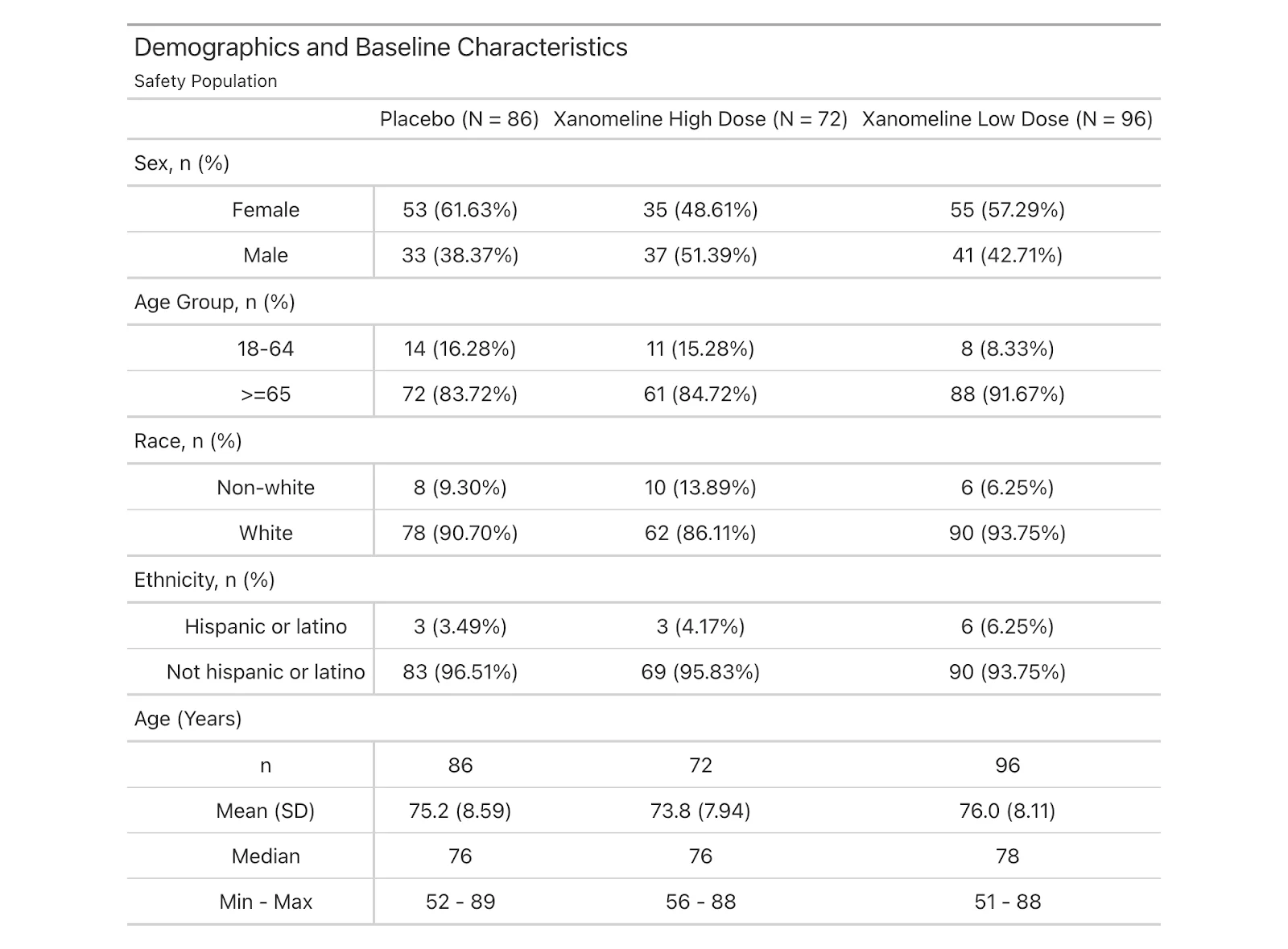
Clinical Trial Demographics and Baseline Characteristics
Discover how Shiny and Quarto are transforming clinical research by exploring our article, “Revolutionizing Clinical Research with Interactive Reports“.
Adverse Events Clinical Table with {gt}
For this table, we will use synthetic adae (ADaM-compliant Adverse Event) data from {chevron} package. We will also calculate the number of subjects for each treatment from the subject-level adsl data.
library(chevron)
library(dplyr)
library(tidyr)
library(gt)

adsl <- syn_data$adsl
adae <- syn_data$adae

number_of_subjects <- adsl |>
  count(ARM, name = "number_of_subjects")

number_of_subjects <- setNames(
  number_of_subjects$number_of_subjects,
  number_of_subjects$ARM
)
Again, we first need to create the table we will supply to the gt function. Each row will represent the number of people with an event, grouped by AEBODSYS (Body System or Organ Class). For each group, we will have overview rows for displaying “Patients with at least one event” and “Total number of events”. Columns will represent the treatments.
Let’s first calculate the number of people and percentages grouped by AEBODSYS. This data will serve as a skeleton for the additional overview rows.
adverse_event_table <- adae |>
  group_by(ARM, AEBODSYS, AEDECOD) |>
  summarise(
    n = n_distinct(USUBJID),
  ) |>
  mutate(
    pct = n / number_of_subjects[ARM]
  ) |>
  pivot_wider(names_from = ARM, values_from = c(n, pct)) |>
  rename(
    groupname = AEBODSYS,
    rowname = AEDECOD
  ) |>
  ungroup()
For the sake of simplicity, let’s write a function that calculates the overview rows either for each AEBODSYS or for all data. Then, use this function to calculate both situations and save the results.
adae_summary <- function(adae, by_aebodsys = TRUE) {
  group_vars <- c("ARM")
  if (by_aebodsys) {
    group_vars <- append(group_vars, "AEBODSYS")
  }
  summarised_data <- adae |>
    group_by(across(all_of(group_vars))) |>
    summarise(
      `Total number of events` = n(),
      `Patients with at least one event` = n_distinct(USUBJID)
    ) |>
    pivot_longer(
      cols = c(`Patients with at least one event`, `Total number of events`),
      names_to = "AEDECOD",
      values_to = "n"
    ) |>
    mutate(
      pct = ifelse(
        AEDECOD == "Patients with at least one event",
        n / number_of_subjects[ARM],
        NA
      )
    ) |>
    pivot_wider(names_from = ARM, values_from = c(n, pct))

  if (by_aebodsys) {
    summarised_data |>
      rename(
        groupname = AEBODSYS,
        rowname = AEDECOD
      )
  } else {
    summarised_data |>
      rename(
        rowname = AEDECOD
      ) |>
      mutate(
        groupname = ""
      )
  }
}

aebodsys_summary <- adae_summary(adae)
total_summary <- adae_summary(adae, by_aebodsys = FALSE)
We will bind summary data frames with the skeleton data frame in the order we want it to appear in the final output.
adverse_event_table <- adverse_event_table |>
  bind_rows(aebodsys_summary) |>
  arrange(groupname, rowname)

final_table <- total_summary |>
  bind_rows(adverse_event_table)
Now just like we did in the demographics table example, we first format the columns, then, merge them, and finally style the table.
final_table |>
  gt(
    rowname_col = "rowname",
    groupname_col = "groupname"
  ) |>
  fmt_percent(
    columns = starts_with("pct"),
    decimals = 1
  ) |>
  fmt_integer(
    columns = starts_with("n_"),
  ) |>
  cols_merge_n_pct(
    col_n = "n_A: Drug X",
    col_pct = "pct_A: Drug X"
  ) |>
  cols_merge_n_pct(
    col_n = "n_B: Placebo",
    col_pct = "pct_B: Placebo"
  ) |>
  cols_merge_n_pct(
    col_n = "n_C: Combination",
    col_pct = "pct_C: Combination"
  ) |>
  cols_label_with(
    fn = \(x) {
      treatment <- stringr::str_remove(x, "n_") paste0(treatment, " (N=", number_of_subjects[treatment], ")") } ) |>
  tab_stub_indent(
    rows = everything(),
    indent = 5
  ) |>
  opt_align_table_header(align = "left") |>
  cols_align(
    align = "center",
    columns = everything()
  ) |>
  tab_header(
    title = "Adverse Events Table"
  )
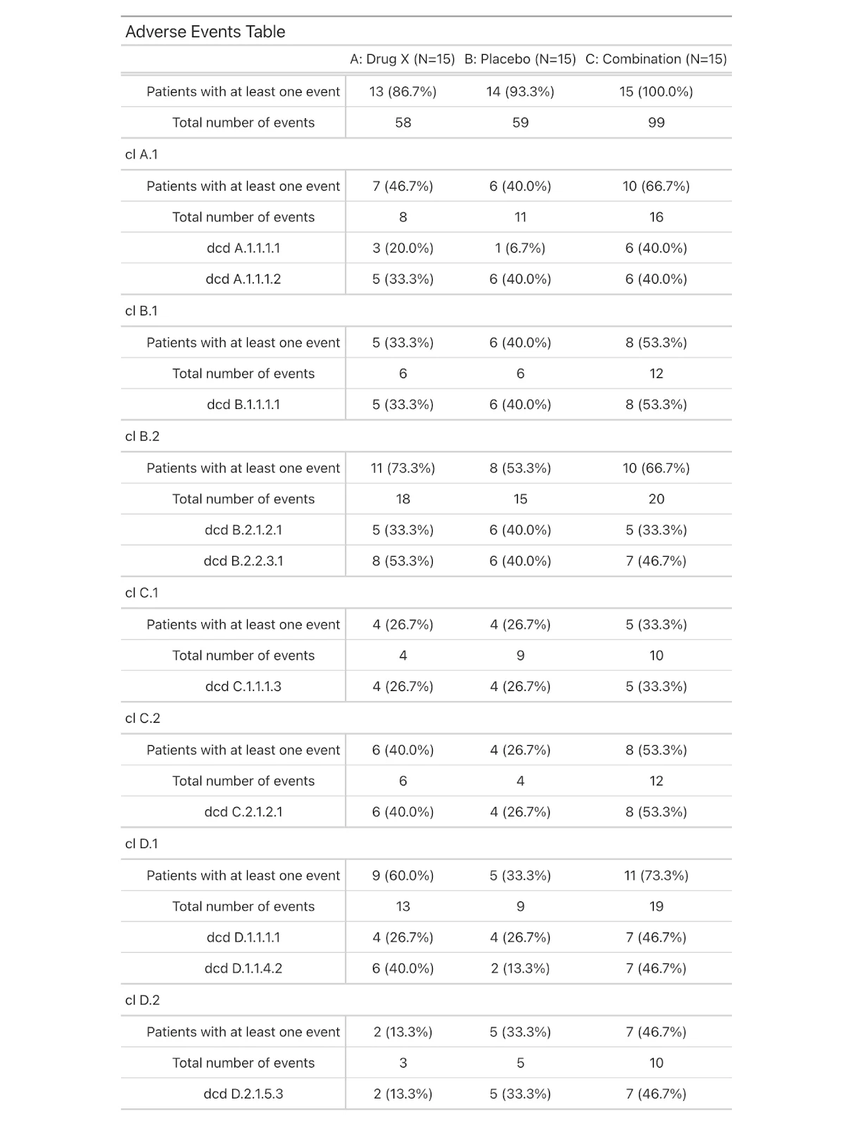
Adverse Events in Clinical Trial
Elevate your regulatory submissions; delve into our guide ‘Reproducible and Reliable Shiny Apps for Regulatory Submissions.
Summing up Clinical Tables with {gt}
The {gt} package is essential for creating detailed and visually appealing tables in clinical trials, aiding in the clear and effective communication of complex data to researchers, clinicians, and stakeholders.
The workflow for creating clinical tables with gt is:
- Preparing the skeleton of the final output by summarizing and cleaning the data.
- Creating the initial table with
gtfunction and specifying therowname_colandgroupname_colarguments. - Formatting columns with
fmt_*functions. - Merging columns with
cols_merge*functions. - Adding final touches by renaming original column names and styling the table.
The R Consortium and {gt} documentation also provide valuable examples and information on clinical tables. I encourage you to experiment with them as well to get familiar with the topic.
We’re looking forward to seeing you at PHUSE US Connect 2024! We will be at Booth 17; join us for engaging conversations and connections with our team.
