Top 10 Machine Learning Evaluation Metrics for Regression – Implemented in R

It’s one thing to train a machine learning model, but how can you know it’s any good? That’s where evaluation metrics come into play. Today, we bring you the top 10 machine learning evaluation metrics for the regression datasets, implemented from scratch in R. We’ll go over the theory, mathematical formulas, and R code first, and then we’ll train a machine learning model and use these metrics to evaluate its performance.

Make sure to stay tuned to the Appsilon blog, as we’ll soon release a similar article regarding classification datasets. All of the metrics you’ll see can be calculated by calling some R function or referring to a specialized package, but we’ll implement everything from scratch. This way, you’ll get a much better understanding of the topic. So without much ado, let’s dive into the good stuff.

Practical Machine Learning Use-Case – Counting Nests of Shags with YOLO.

Table of contents:

• Machine Learning Evaluation Metrics for Regression – From Theory to Implementation
• Using Regression Evaluation Metrics on a Real Dataset – A Machine Learning Use-Case
• Summing Up Machine Learning Evaluation Metrics for Regression

Machine Learning Evaluation Metrics for Regression – From Theory to Implementation

This portion of the article will walk you through the top 10 machine learning evaluation metrics for regression, from background and theory to mathematical formulas and R code implementation. We’ll start with the most obvious one – Mean Absolute Error.

1. Mean Absolute Error (MAE)

The Mean Absolute Error metrics measures the average absolute difference between predicted and actual values. You can calculate it by taking the absolute value of the difference between the predicted and actual values, and then taking the average across all samples.

This metric is popular among data scientists and machine learning engineers because it’s easy to interpret – it just tells you how off your regression model is on average.

Take a look at the mathematical formula:

Image 1 – Mean Absolute Error formula

It’s not that difficult to replicate in R programming language, but if you get stuck, just copy our code snippet:

MAE <- function(y, y_pred) {
  mean(abs(y - y_pred))
}

2. Mean Squared Error (MSE)

Mean Squared Error is almost identical to Mean Absolute Error, but with one critical difference – it measures the squared difference between actual and predicted values instead of the absolute difference.

Squaring penalizes larger errors more heavily than smaller errors, which is frequently the behavior you want when training machine learning models. Because of this reason, MSE is the most common loss function used in machine learning.

Keep in mind that MSE returns the error in units squared, so it’s a bit trickier to interpret. For example, if you’re predicting housing prices in thousands of dollars, MSE will return an error in the unit of thousands of dollars squared. Taking a square root from the calculation is the best next step if you care for interpretability, and that’s where the next metric comes in.

Take a look at the mathematical formula:

Image 2 – Mean Squared Error formula

If you want R implementation, here’s one approach that works:

MSE <- function(y, y_pred) {
  mean((y - y_pred)^2)
}

3. Root Mean Squared Error (RMSE)

The Root Mean Squared Error metric does everything MSE does, but it makes the error more interpretable by bringing the value to the original units. If you’re predicting age, it makes no sense to interpret the error in pounds or kilograms squared, as it’s just confusing.

RMSE still penalizes larger errors like MSE but takes an additional step of bringing the error values back to the original unit.

Take a look at the mathematical formula:

Image 3 – Root Mean Squared Error formula

R implementation is also straightforward:

RMSE <- function(y, y_pred) {
  sqrt(mean((y - y_pred)^2))
}

4. Root Mean Squared Log Error (RMSLE)

The Root Mean Squared Log Error metric is similar to RMSE, but it takes the logarithm of the predicted and actual values before calculating the squared difference. It is used oftentimes when the target variable has a wide range of values.

The RMSLE function first takes the natural logarithm of the predicted values and actual values and then calculates the squared differences between them. Once done, it calculates the RMSE based on the logarithmic difference.

Take a look at the mathematical formula:

Image 4 – Root Mean Squared Error formula

R implementation is easy, just be careful with the brackets:

RMSLE <- function(y, y_pred) {
  sqrt(mean((log(y_pred + 1) - log(y + 1))^2))
}

5. R-squared (R2)

The R-squared metric, sometimes also called Coefficient of Determination measures how much variable in the target variable is explained by the machine learning model. The possible values range from 0 to 1, larger being better, and 1 meaning the line perfectly fits the data.

R-squared is calculated by dividing the variance of the predicted values by the variance of actual values.

Take a look at the mathematical formula:

Image 5 – R-squared formula

If you prefer R over math, here’s the code snippet for you:

R2 <- function(y, y_pred) {
  1 - sum((y - y_pred)^2) / sum((y - mean(y))^2)
}

6. Mean Absolute Percentage Error (MAPE)

The Mean Absolute Percentage Error measures the average percentage difference between predicted and actual values. You can calculate MAPE by taking the absolute value of the difference between the predicted and actual values, and then divide these by the actual values, and finally take the average across all samples.

It’s quite a process, but you’ll see that the implementation is mostly straightforward. The MAPE metric is oftentimes used when the target variable is expressed as a percentage and has a non-zero mean, so keep that in mind.

Take a look at the mathematical formula:

Image 6 – Mean Absolute Percentage Error formula

Implementation in R is close to effortless, especially if you consider all the steps described in the first paragraph:

MAPE <- function(y, y_pred) {
  mean(abs((y - y_pred) / y)) * 100
}

7. Symmetric Mean Absolute Percentage Error (SMAPE)

The Symmetric Mean Absolute Percentage Error is quite similar to MAPE, but it can handle zero values. You can calculate it by first taking the absolute value of the difference between the predicted and actual values, then dividing the sum of the predicted and actual values, and finally multiplying it by 2 and taking the average across all samples.

Once again, it’s quite a few steps, but the metric is useful for all cases in which you would use MAPE, and also when the target variable can be zero.

Take a look at the mathematical formula:

Image 7 – Symmetric Mean Absolute Percentage Error formula

From-scratch implementation in R is quite straightforward if you understand the formula:

SMAPE <- function(y, y_pred) {
  mean(2 * abs(y - y_pred) / (abs(y) + abs(y_pred))) * 100
}

8. Mean Directional Accuracy (MDA)

The Mean Directional Accuracy metric is quite a unique one, as it measures the percentage of correct predictions in terms of the direction of change (up or down).

You can calculate it by counting the number of times the predicted value has the same sign as the actual value divided by the total number of samples. Easy enough, but the formula might look scary at first:

Image 8 – Mean Directional Accuracy formula

R implementation also isn’t the easiest to read, especially if you want to condense the code into a single line:

MDA <- function(y, y_pred) {
  mean(sign(y[2:length(y)] - y[1:(length(y) - 1)]) == sign(y_pred[2:length(y_pred)] - y[1:(length(y) - 1)]))
}

9. Median Absolute Error (MedAE)

Let’s now take a break from these complicated equations and cover a simple and intuitive metric – Median Absolute Error. It’s almost identical to MAE, but it calculates the median over the mean.

For this reason, MedAE is less sensitive to outliers. Take a look at the formula:

Image 9 – Median Absolute Error formula

Implementing MedAE in R requires almost no effort:

MedAE <- function(y, y_pred) {
  median(abs(y - y_pred))
}

10. Explained Variance Score (EVS)

And finally, let’s discuss Explained Variance Score. This metric measures the proportion of variance in the target variable that is explained by the model. You can calculate EVS by taking the difference between the variance of the actual values and the variance of the residuals, and then divide by the variance of the actual values. The values for this metric range from 0 to 1, where 1 indicates a perfect fit to the data.

Take a look at the formula:

Image 10 – Explained Variance Score formula

R implementation is easy, as there’s already a var() function built-in:

EVS <- function(y, y_pred) {
  1 - var(y - y_pred) / var(y)
}

Using Regression Evaluation Metrics on a Real Dataset – A Machine Learning Use-Case

By now, you should be familiar with the machine learning evaluation metrics for regression we’ve described in the previous section. You don’t have to be an expert, of course, just be aware of what the metric stands for and what’s the possible value range.

In this section, we’ll shift focus on training a machine learning model from scratch and using the previously implemented regression metrics to evaluate the model.

This is not a comprehensive section on machine learning. Our goal is to train the model as fast as possible so we can focus on evaluation using the regression metrics. For more in-depth guides on machine learning, check out our recent articles.

Dataset Loading and Preparation

We’ll keep things simple and use the well-known Boston Housing Dataset. You don’t have to download it, as it’s built into the R’s MASS package. You might have to install the package, though.

First, let’s import the dataset and see what it looks like:

library(MASS)
library(caret)

data(Boston)
df <- Boston
head(df)

Here are the first six rows, returned by the head() function:

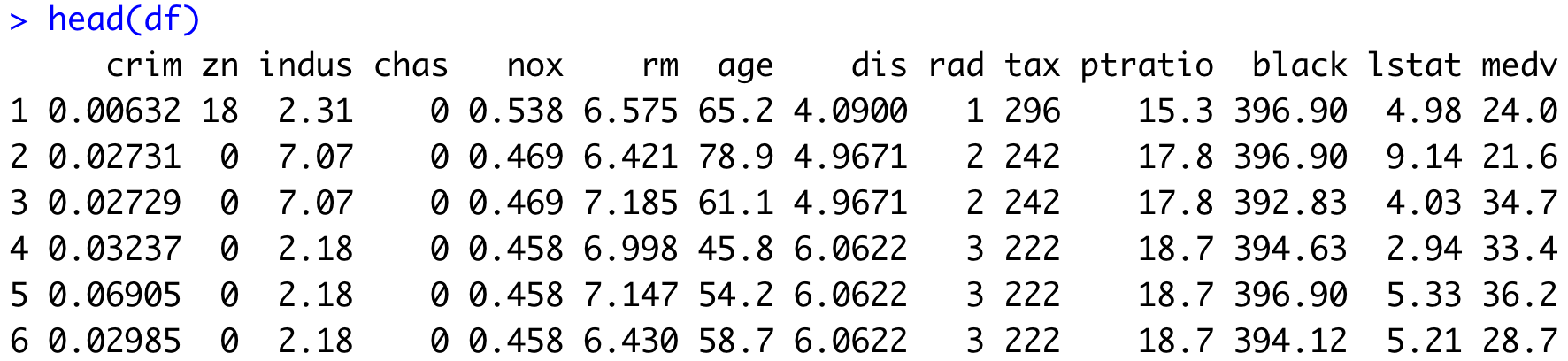
Image 11 – Head of the Boston Housing Prices dataset

For simplicity’s sake, we’ll remove all rows that have any missing values. This should be a problem since the dataset is tailored toward machine learning newcomers:

# Remove all rows with missing values
df <- df[complete.cases(df), ]

Train/Test Split

The goal of a dataset split into training and testing subsets is to have a small portion of the data that was never seen by the predictive model. This way, we can monitor how the model behaves on previously unseen data.

The standard procedure is to have 80% of the data in the training set, and 20% in the testing set. Here’s how to implement that in R:

set.seed(123)
trainIndex <- createDataPartition(df$medv, p = 0.8, list = FALSE)
train <- df[trainIndex, ]
test <- df[-trainIndex, ]

dim(train)
dim(test)

The dim() function prints the dimensionality of a data.frame (number of rows, number of columns):

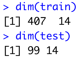
Image 12 – Dimensionality of training and testing sets

Dataset Standardization

Finally, let’s talk about standardization. It’s a step you shouldn’t skip because most machine learning algorithms expect to have data on the same scale. For example, if one feature ranges from 1 to 10, and the other from 1000 to 10000, a machine learning model might think the second feature is more important. It obviously isn’t, and standardization is here to tell the model that.

We’ll use the caret R package to center and scale the values in both sets, as implemented via the following snippet:

# Standardize the variables
preProcValues <- preProcess(train[, -ncol(train)], method = c("center", "scale"))
train[, -ncol(train)] <- predict(preProcValues, train[, -ncol(train)])
test[, -ncol(test)] <- predict(preProcValues, test[, -ncol(test)])

The last step is to ensure the target variable is numeric in both sets. You can do so by applying the as.numeric() function on the column:

# Ensure the target variable is numeric
train$medv <- as.numeric(train$medv)
test$medv <- as.numeric(test$medv)

Let’s check the structure of the training set to verify everything looks correct:

str(train)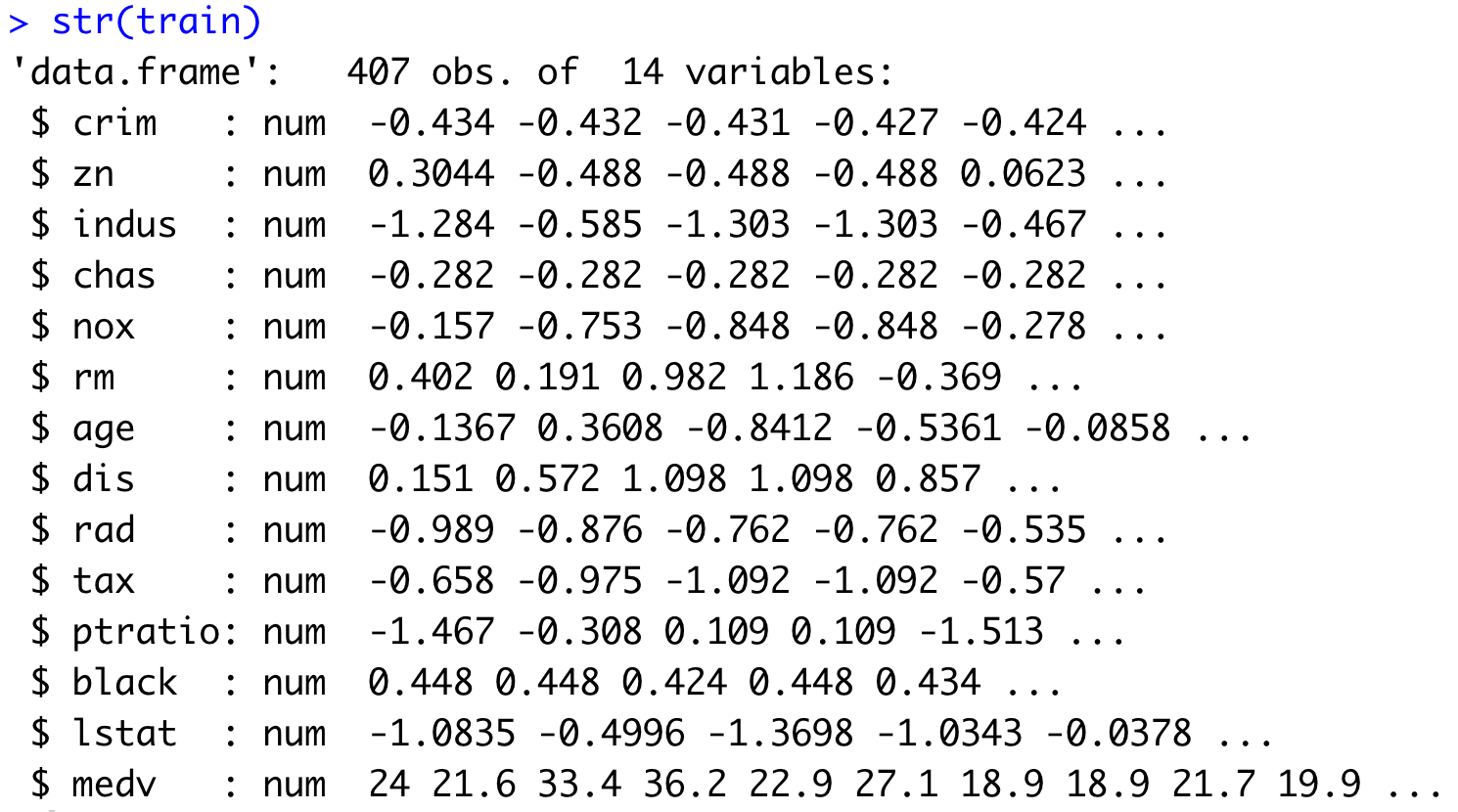

Image 13 – Structure of the training set

All variables are numeric, and all predictors (not the target variable) are on the same scale.

Let’s continue by training a machine learning model.

Training a Machine Learning Model

R makes it incredibly easy to train a regression model. All we have to do is to call the train() function on our training dataset, and specify we want to predict medv based on all of the available features.

The following code snippet trains the model and prints its summary:

model <- train(medv ~ ., data = train, method = "lm")
summary(model)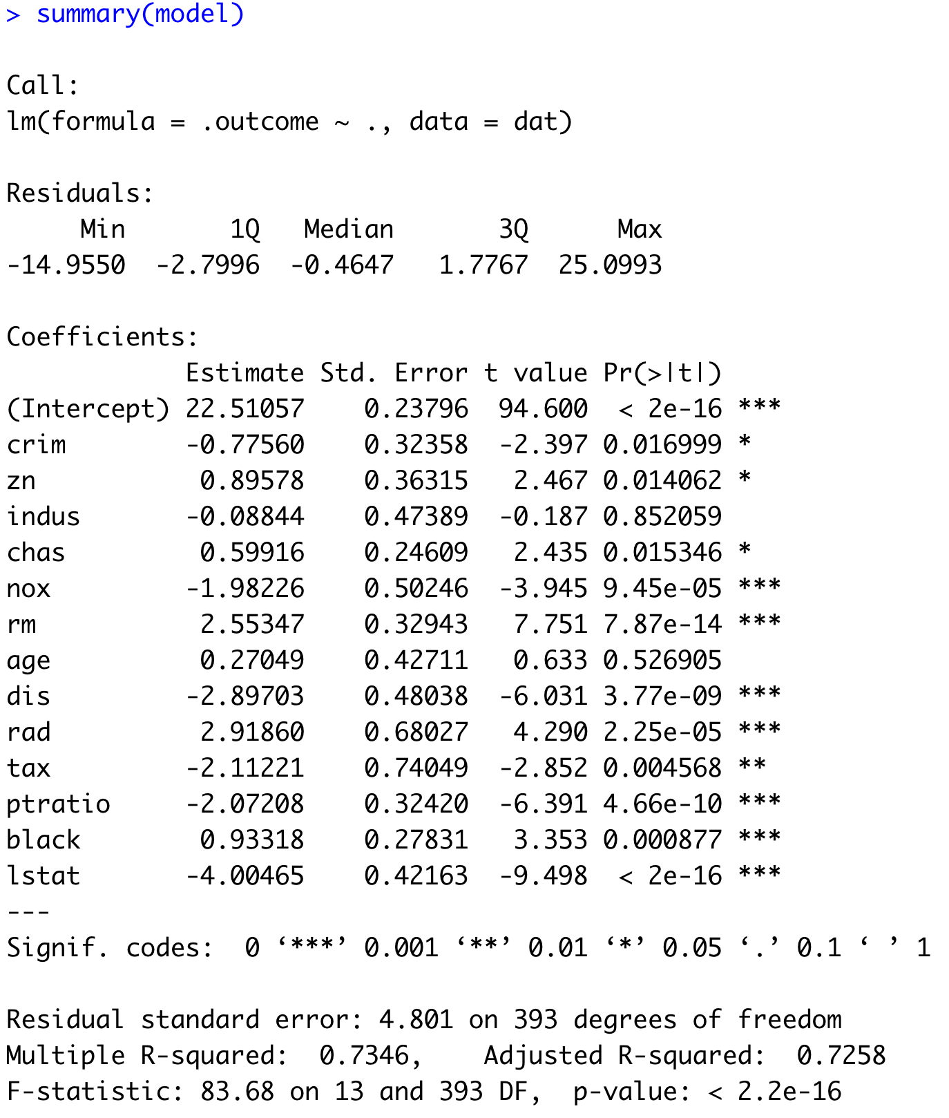

Image 14 – Machine learning model summary

If you see a star next to the feature name, it means the given feature is important for the model’s predictive performance. How important? The number of stars determines that. The more stars the feature has, the lower the P-value, and hence the more impact the feature has on the overall prediction.

We’ll now use this model to make predictions on the test set:

predictions <- predict(model, newdata = test)
predictions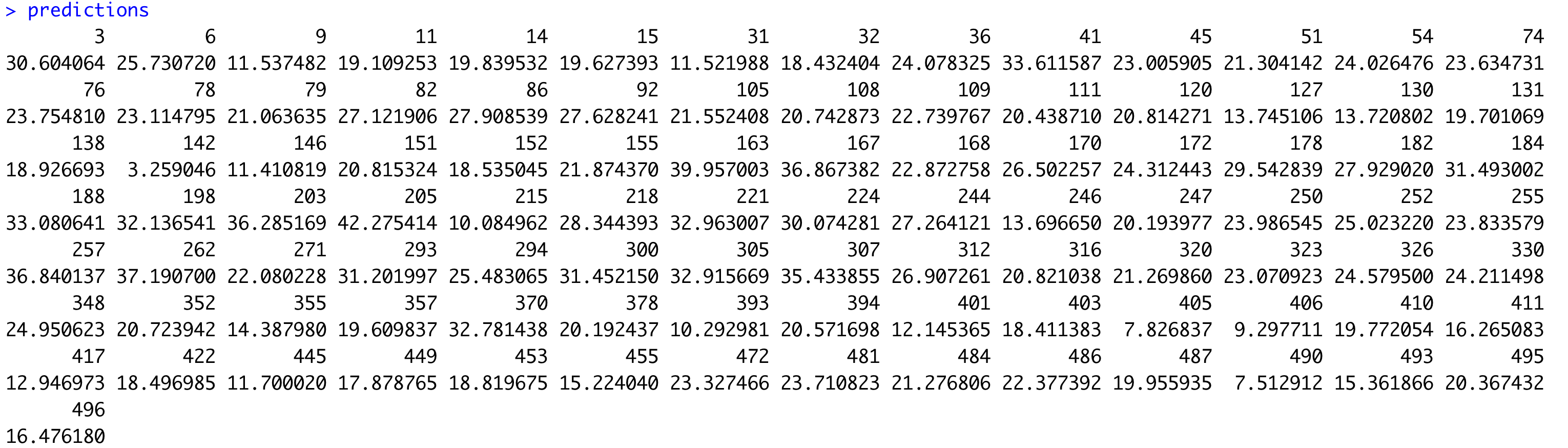

Image 15 – Test set predictions

These are the values we’ll use to evaluate the model with our choice of 10 regression metrics.

Machine Learning Evaluation Metrics for Regression in Action

This is the part you’ve been waiting for. We’ll now finally use our 10 R functions to calculate the values of regression metrics.

One approach is to make a data.frame of regression metrics, just so we don’t have to print each one manually. Here’s the code snippet:

dfEvalMetrics <- data.frame(
  "MAE"   = MAE(y = test$medv, y_pred = predictions),
  "MSE"   = MSE(y = test$medv, y_pred = predictions),
  "RMSE"  = RMSE(y = test$medv, y_pred = predictions),
  "RMSLE" = RMSLE(y = test$medv, y_pred = predictions),
  "R2"    = R2(y = test$medv, y_pred = predictions),
  "MAPE"  = MAPE(y = test$medv, y_pred = predictions),
  "SMAPE" = SMAPE(y = test$medv, y_pred = predictions),
  "MDA"   = MDA(y = test$medv, y_pred = predictions),
  "MedAE" = MedAE(y = test$medv, y_pred = predictions),
  "EVS"   = EVS(y = test$medv, y_pred = predictions)
)
t(dfEvalMetrics)

And here are the results:

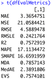
Image 16 – Values of the regression evaluation metrics

On average, our predicted value is 4.6 units wrong when compared to the actual values (RMSE). In percentage terms, that’s roughly 17% (MAPE). The regression model “line” covers approximately 75.7% of the variance from the data.

Summing Up Machine Learning Evaluation Metrics for Regression

And there you have it – the most comprehensive guide on machine learning evaluation metrics for regression in R. We’ve covered all of the metrics we work with daily, and explained them with theory, math, and R programming language implementation.

We hope this article gave you a clear picture of how easy it is to implement these metrics from scratch, and that you’ve also gained a deeper understanding of the math and overall logic.

What are your favorite machine learning evaluation metrics for regression? Are there any we’ve left out? Make sure to let us know in the comment section below. Or even better – reach out on Twitter – @appsilon. We’d love to hear your feedback.

Are you up for a challenge? Here are 5 R-based take-home challenges for Data Scientists. How many can you solve?