R Docker: How to Run Your R Scripts in a Docker Container

So, you’ve written this amazing R script, but your coworkers can’t run it? It works on your machine, so they have to be doing something wrong, right? Wrong. It’s all about isolating and managing R environments.

And that’s where R Docker comes in. Think of Docker as a program that allows you to run multiple operating systems (containers) on your machine, while also allowing you to share the blueprints for recreating the mentioned operating system. It’s like a virtual machine, minus everything you don’t need.

Today you’ll learn the basics of R Docker, why it’s important in R programming language, and how to Dockerize your first R script.

Is your R Shiny app slow? You might want to consider scaling it at the infrastructure level.

Table of Contents

• What is Docker and Why is it Important in R Programming
• How to Install Docker
• How to Use R Docker to Run R Script in a Container
• Summing up R Docker

What is Docker and Why is it Important in R Programming

Think of Docker as a platform for developing, shipping, and running applications in isolated environments called “containers”. These are lightweight units that package applications and all of their dependencies (think system dependencies and R packages).

In the context of R programming, Docker addresses the problem of environment consistency. Needless to say, you want your code running consistently across different environments, from your laptop to production servers. Docker containers can help here, as they encapsulate the environment, so you can rest assured the code and dependencies won’t change as you change the development environment.

Docker is also praised for the reproducibility aspect. They allow you not only to specify which R dependencies are needed but also specific versions of R itself and other system dependencies. This will ensure you don’t run into any issues when sharing your code with others. If it works on your laptop (in a Docker container, of course), it will work with other developers as well.

The previous two points also give you the idea that Docker containers benefit from portability. You can create a container on your laptop and then run it on any platform that supports Docker, such as your other laptop, a cloud server, or even a home NAS system.

And, of course, Docker makes scaling R applications a breeze. You can create multiple containers with the same configuration and scale your application horizontally as the workload increases.

There are other benefits of using R Docker, but we think these few are enough to convince you Docker is the correct way of creating and scaling R scripts and applications.

But how can you install Docker? That’s what we’ll cover next.

How to Install Docker

If you’re working on a PC/laptop, we recommend installing Docker Desktop:

Image 1 – Docker homepage

Put simply, it’s a single .exe file for Windows, .dmg file for Mac, and .deb/.rpm file for Linux you can download at the URL supplied earlier.

Just download the file and install it with a double click (Windows and Mac), or by running the following shell commands on Linux:

sudo apt-get update
sudo apt-get install ./docker-desktop-<version>-<arch>.deb

Installation on Mac and Windows is easier, so we feel there’s no need to discuss it further. Linux might require some additional tweaking, so feel free to go over the official installation instructions.

How to Use R Docker to Run R Script in a Container

This section will walk you through the process of writing a simple R script, and then automating its execution in a Docker container.

Writing and Testing the R Script

This is likely your first introduction to Docker, so let’s not overcomplicate things where we don’t have to. We’ll keep the R portion fairly simple.

Create a new R script file (ours is named script.R). It uses two external dependencies – dplyr and gapminder to load and summarize a dataset.

To be more precise, the script gives us insights into average life expectancy and average GDP per capita for all European countries in 2007.

The results are saved to a CSV file. Note the save path, this one is important for later:

library(dplyr)
library(gapminder)

# Statistics of Europe countries for 2007
eu_stats <- gapminder %>%
  filter(
    continent == "Europe",
    year == 2007
  ) %>%
  group_by(country) %>%
  summarise(
    AvgLifeExp = mean(lifeExp),
    AvgGdpPercap = mean(gdpPercap)
  )

# Save the file as CSV
write.csv(eu_stats, "home/r-environment/eu_stats.csv", row.names = FALSE)

This is what you’ll see once you run the script locally:

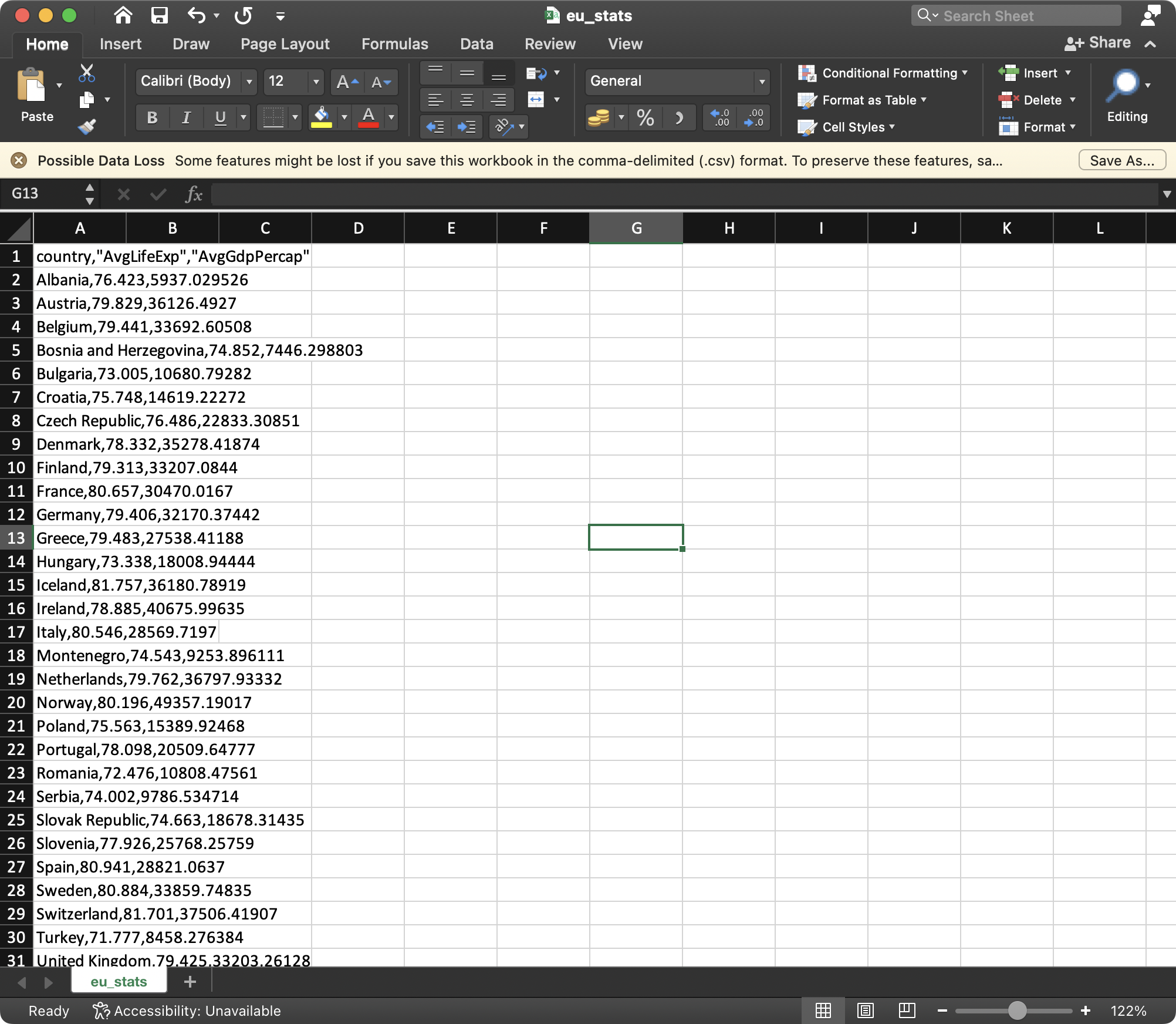
Image 2 – The resulting CSV file

Nothing fancy and nothing to write home about – but does the job. Running the script results in an output CSV file, which will be a verification to make sure things work properly when executed in a Docker container.

Let’s see how to approach this next.

Writing the Dockerfile

We’ll leverage a Dockerfile to create our container for the R script. Create a new file in the same directory where your R script is, and name it Dockerfile – all one word, no extensions.

This type of file uses a specific syntax to create a Docker container. Let’s go over a couple of common keywords:

• FROM: A command every Dockerfile starts with. It’s used to describe what base image are we building our image from. For example, rocker/r-ver is built on Ubuntu LTS and installs a fixed version of R from source. You can specify the exact version of R by putting :<r-version> after rocker/r-ver. Feel free to explore the details of this image further on your own.
• RUN: This command mimics command line commands, and we can use them to do things such as directory creation, dependency installation, and much more.
• COPY: A command used to copy the contents of your local machine to the container. Use the syntax COPY <path-tolocal-file> <path-in-container>, or replace <path-tolocal-file> with . to copy everything from the folder.
• CMD: This is the command that will be used every time you launch the container. For example, we can use it to run our R script.

There are more keywords you can use, but these will be enough for today.

Here are the Dockerfile contents, so feel free to copy-paste them:

# Base R image
FROM rocker/r-ver

# Make a directory in the container
RUN mkdir /home/r-environment

# Install R dependencies
RUN R -e "install.packages(c('dplyr', 'gapminder'))"

# Copy our R script to the container
COPY script.R /home/r-environment/script.R

# Run the R script
CMD R -e "source('/home/r-environment/script.R')"

In a nutshell, we’re using the latest version of the r-ver image, creating a directory, installing R dependencies, copying the local script to the container, and running it.

That’s it! The syntax takes some time to get used to but is simple and readable. You’ll have more trouble writing than reading Dockerfile if you’re just starting out.

Creating a Docker Container and Running the Script

We’re only two shell commands away from running our R script in a Docker container.

The first shell command is used to build a container per your Dockerfile instructions. Open up a new Terminal window and navigate to where your code is located. Then, run the following command:

docker build -t r-docker-demo .

This will build a new image named r-docker-demo:

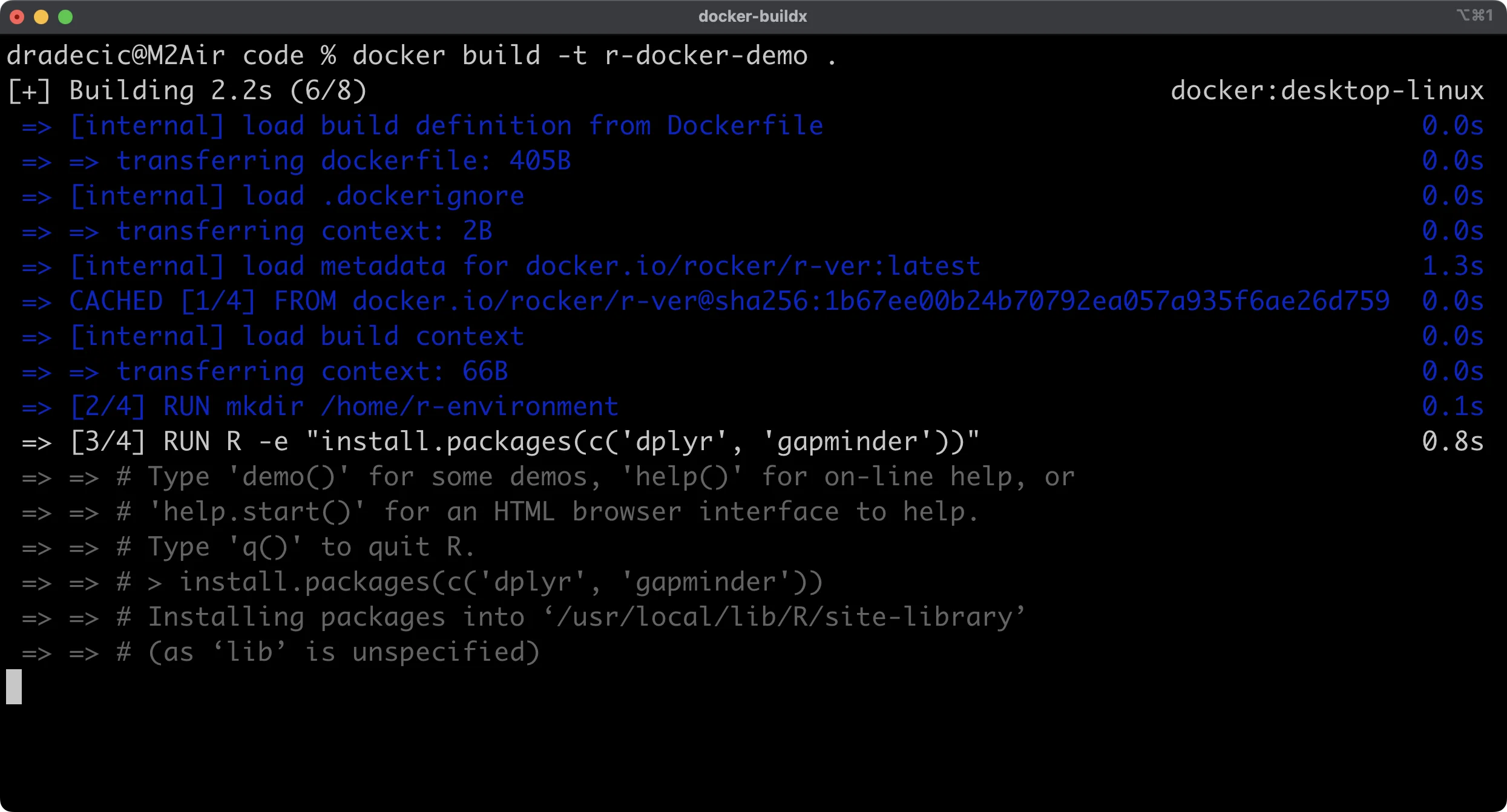
Image 3 – Building a container from Dockerfile

You’ll see this message when the build finishes:

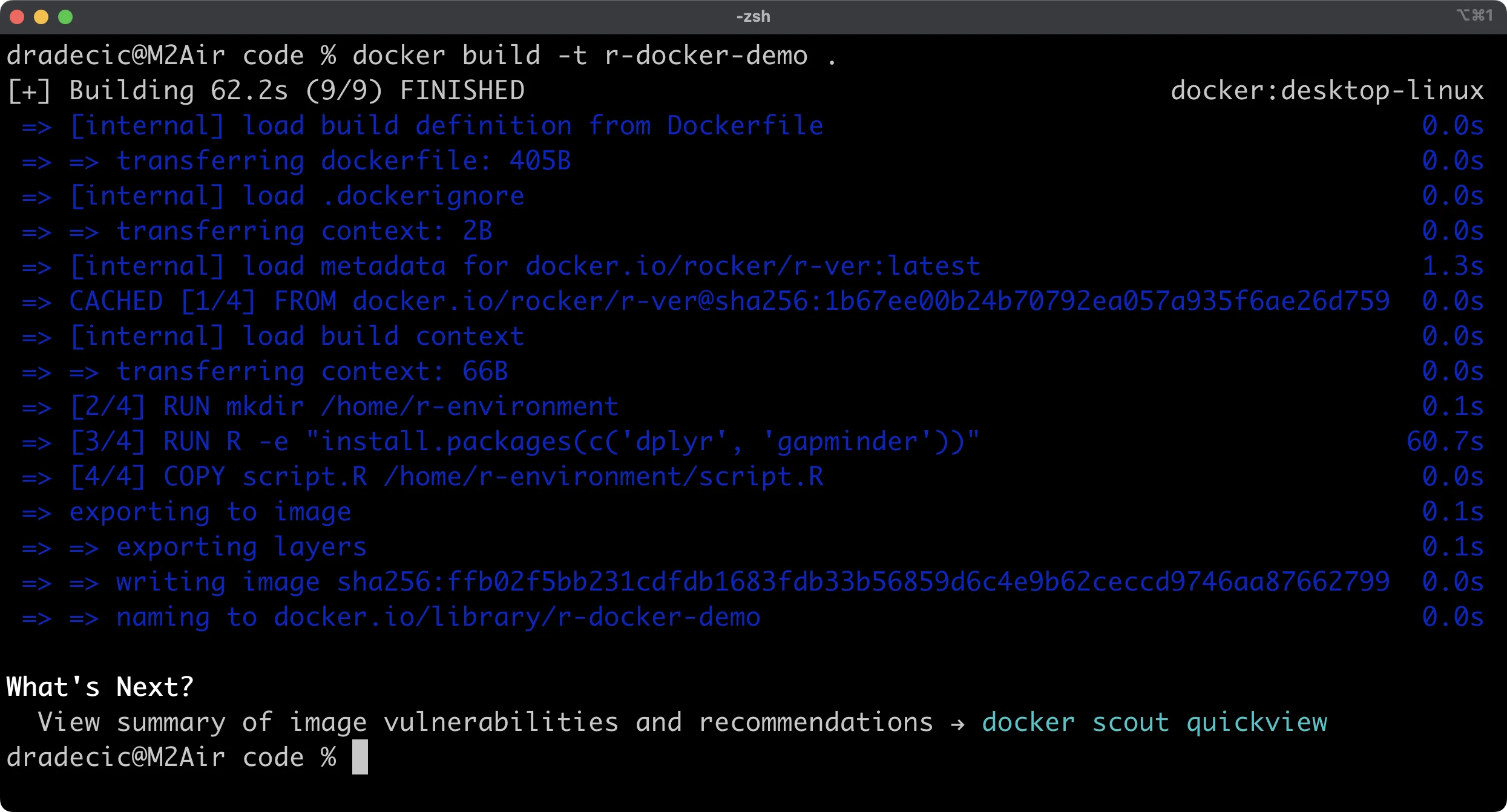
Image 4 – Container build finished

And now, we can finally create a container from the newly created image and run it:

docker run r-docker-demo

This is the shell output you’ll see:

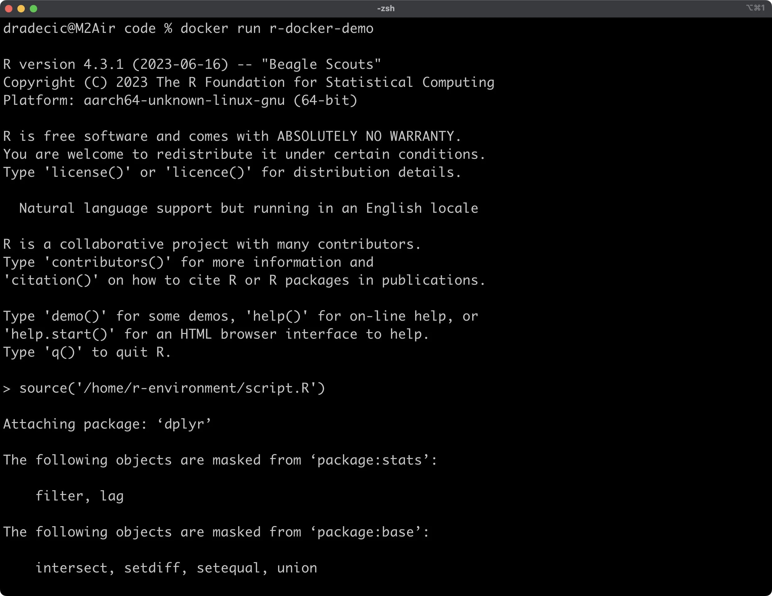
Image 5 – Launching a Docker container

You can see the runtime logs by opening Docker Desktop and monitoring container runs. You’ll see the identical output as previously shown in Terminal:

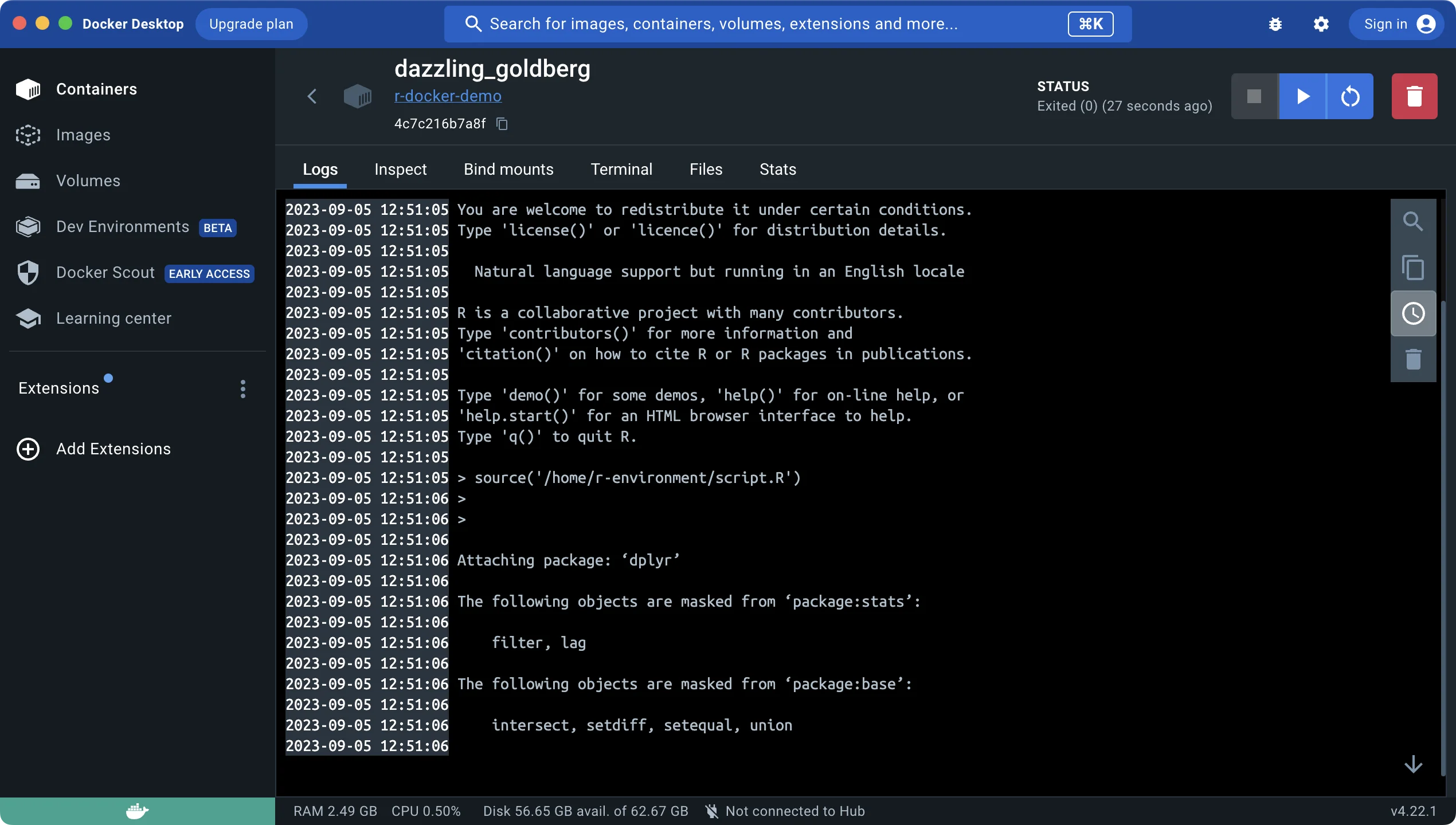
Image 6 – Docker container log output

The Files tab is where things get interesting. Long story short, this tab provides you with an overview of the system file structure.

If our R script finished successfully, we should see an eu-stats.csv file stored in home/r-environment:

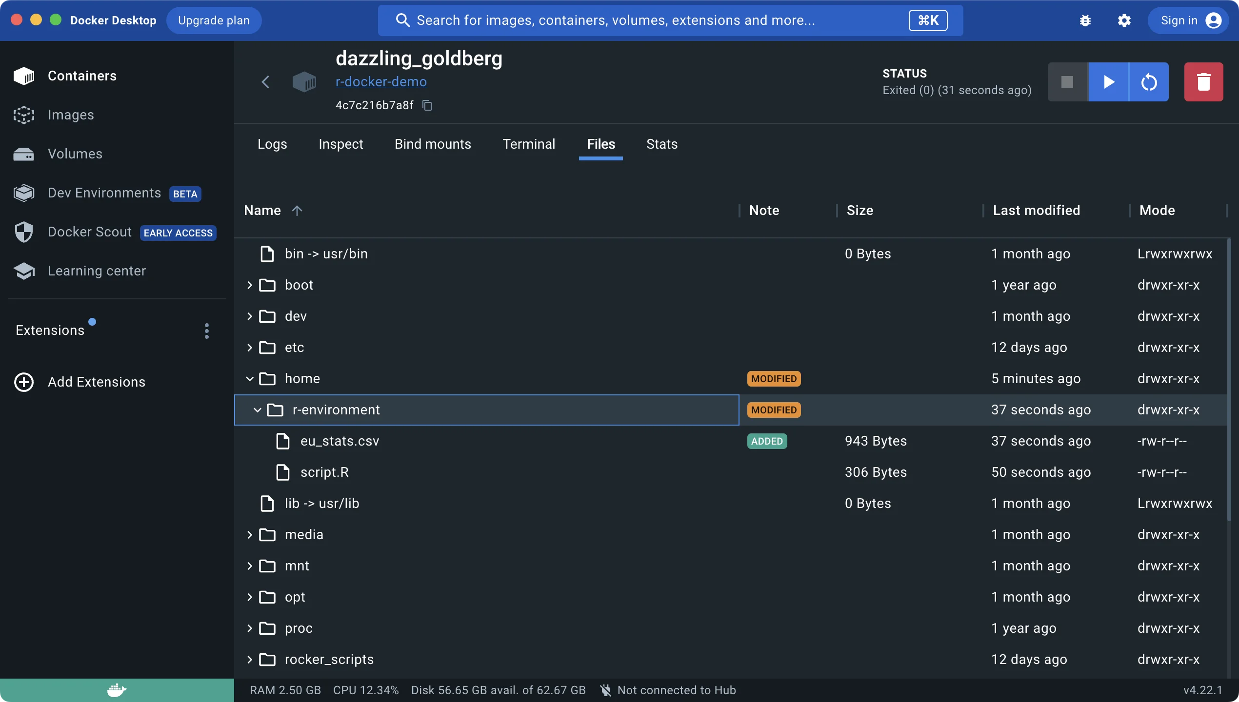
Image 7 – Docker container system files

You can download this file locally to your system:

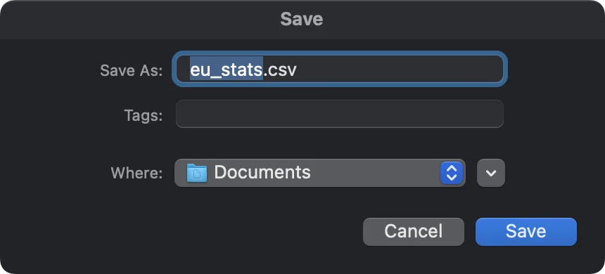
Image 8 – Saving the container file locally

And here’s what it contains:

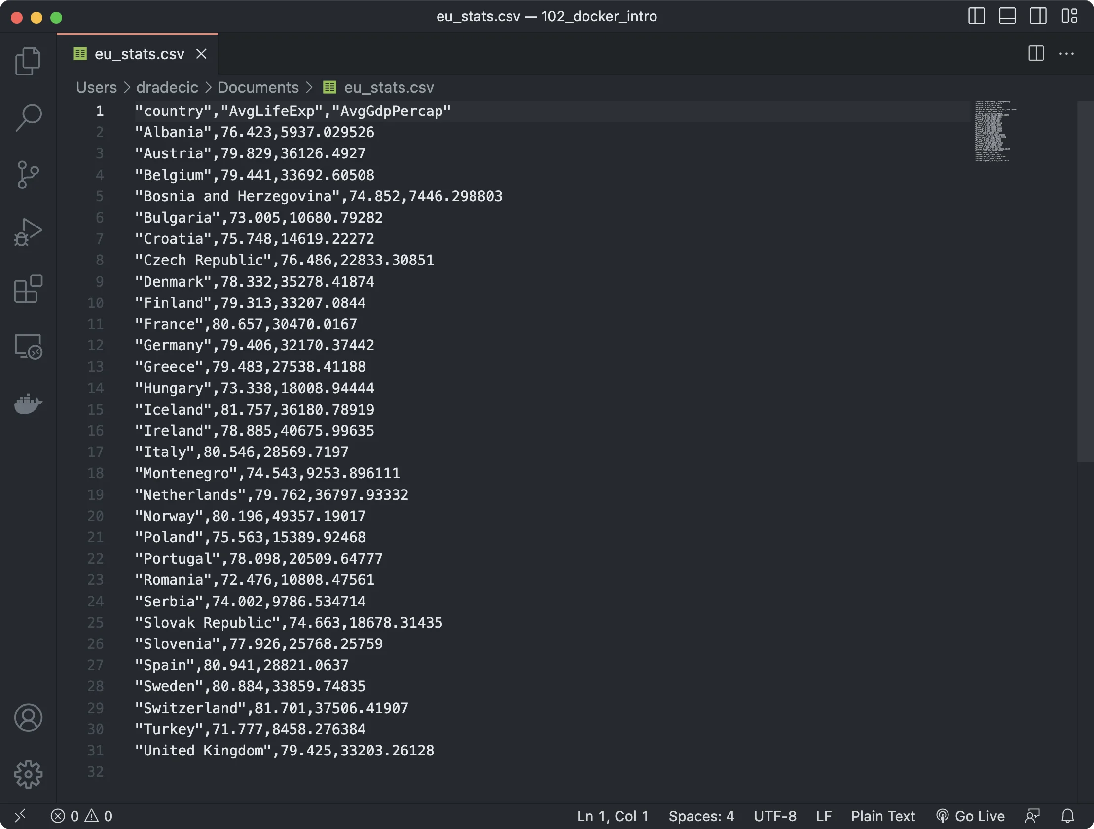
Image 9 – Resulting CSV file contents

To conclude, we’ve successfully written and Dockerized a simple R script. You can share the script and Dockerfile with your colleagues, and they’ll have no trouble reproducing your results.

That’s the whole point, after all.

Summing up R Docker

And there you have it – your first Dockerized R script. It takes some time to get used to writing Dockerfiles, but it’s nothing you can’t wrap your head around if you already understand more complex topics, such as programming.

Today you’ve only Dockerized one R script, so the next step is to explore how to do the same (and more) with an entire R Shiny application. Make sure to stay tuned to Appsilon Blog if you want to learn more about deployment.

What’s your preferred way of deploying and sharing R scripts and Shiny applications? Let us know in the comment section below.

Is your R Shiny application slow? Speed it up by offloading heavy calculations with shiny.worker.