During the pandemic, the supply chain and its management strategy burst into the spotlight. Supply chain management (SCM) became a household topic as its disruptions began to directly impact people’s lives and the global economy.
But the truth is, good supply chain strategies are the ones that are aligned with business strategy. And in this complex environment, there is a trade-off between responsive versus efficient strategies.
- Spreadsheets, R, and Supply Chain Management
- Strategy and the Supply Chain
- Supply Chain Overview
- R and Supply Chain Models
- Supply Chain Management in R use case
- Sharing results using R Shiny
Spreadsheets, R, and Supply Chain Management
A spreadsheet solution enables a lot of flexibility but it comes at the expense of reproducibility and error pruning. ERP is a very mature system and has strict rules that make it reliable and efficient but adds little opportunity for newer designs.
This is an extreme example, but it’s a valid one:
Where IT products are not flexible enough nor have the required development speed for business needs, having spreadsheet solutions where an IT product should be used is a common source of strategy misalignment. And one that causes visibility issues in the supply chain.
This is where R comes into play. It’s great for solutions that require a certain degree of development speed and flexible design but are also reproducible with the building blocks of IT maturity. Knowing the requirements that allow an R solution to shine also depends on a proper understanding of where you stand with IT requirements and the business environment.
In this post, we depict the general understanding of business strategy and supply chain as a subsidy to strategic alignment and why using R sustains the visibility and reproducibility required for SCM strategy.
We’ll also show use cases for R and Shiny in SCM and how to add additional value.
Strategy and the Supply Chain
Porter has a great definition of strategy: “the creation of fit between activities, where each activity is consistent, mutually reinforcing, and the fit is done optimally for competitive advantage.”
This fit can have different perspectives such as:
- Internal fit: Organization structure
- External fit: Competition
- Dynamic fit: Demand behavior
Also, Shapiro and Heskett state that strategy has a set of dichotomies that creates tension on each perspective, therefore, strategy decisions will always inherit a set of trade-offs.
This is an extensive field, and for this post, this is an essential concept. If you want to go further, I highly recommend Wharton’s free Strategic Management program.
Supply Chain Overview
The supply chain is a big topic and can be explained through a variety of viewpoints. Below is a condensed summary of the SCOR Model and other descriptions.
An additional summation:
Strategic fit in the Supply Chain
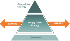
A strategic fit occurs when the competitive strategy and supply chain strategy align goals. Its success is connected to several factors:
- Adjustment between the competitive strategy and functional supply chain strategies
- Proper design of the processes and resources of different functions
- Alignment between supply chain design and the role of each stage
A company can fail because of a lack of strategic fit or because the overall design, supply chain processes, and resources do not provide enough to support the desired strategic outcome.
There are three basic steps to achieve this and overcome potential failure:
- Understand client uncertainty
- Understand the supply chain capacities
- Implement/Set the strategic fit
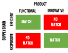
In summary, these steps ensure that there is an appropriate supply chain strategy for each product/service. And functional products have an efficient supply chain strategy while innovative products should fit with a responsive supply chain design. This is called the zone of strategic fit.
Staying competitive
It is important to note that products have a lifecycle, and the supply chain should account for that. Also, the real world is a dynamic system. That’s why alignment with the business strategy is important. It ensures the correct approach under each state of change.
Being able to understand what the drivers of change are and leverage them is what makes supply chain a field of both science and art. This means your supply chain strategy should leverage the theory, but also be fine-tuned for unique situations.
Therefore, using analytic solutions that can leverage both real data and theory into actionable insights provides huge value for supply chain strategists. Reproducibility is a key factor of success because it enhances visibility and enforces alignment between the scope of strategy and operations, as well as maintains sustainability.
For further studies on the supply chain, audit the free MITx program.
R and Supply Chain Models
When we’re abstracting a model or testing a specific problem, using spreadsheets seems a great way to get the work done. Because it is at its core, flexible. But, in this situation, it’s can be difficult to explain the solution to others and make sure that the appropriate workflow is being followed.
Another drawback of spreadsheets is complex logic. When it comes to more complex problems it becomes harder to set the appropriate logic to design the solution in a steady state. Whereas in R, you can leverage a set of best practices and cutting-edge solutions from packages that are maintained by CRAN. This extends the level of quality that R grants to its users.
Note: CRAN is not without its risks. To ensure your project remains secure, you should explore the Isoband Incident and how to mitigate risks.
SCM in spreadsheets vs R example
Let’s take a look at an example by comparing the two solutions: spreadsheets vs R.
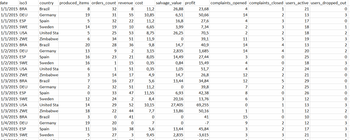
For each of the metrics in the data, you are asked to calculate the change in the sum of all countries in the ongoing previous month and previous year against the current one:
The concept is straightforward, we basically have to:
- Group the data by date and sum each metric to account for all countries
- Calculate the lag from the ongoing previous month and previous year
- Calculate the difference between the lagged previous month/year and the current date.
To do this in spreadsheets, there are many approaches you could work on. One such example:
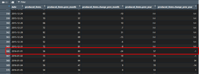
In this example, we can see that on the 1st of January 2016 56 items were produced while on the 1st of December 2015 it produced 80 items. This is a change in production by -24 items. The same logic applies to the year metric.
The data transformation that was asked for is complete. So what’s the issue then?
Reproducibility with spreadsheets
Basically, this approach adds too many manual insertions and each calculation must be checked and updated by the user. There is also the risk of mixing different cells in the calculation, this is the reproducibility problem.
Let’s not forget that we also need 6 other metrics on the data; the same approach is to be repeated 6 times in the spreadsheet.
Imagine for instance that data changes or another metric should be included later on. You will soon enter the spreadsheet productivity dilemma. It was fast to design, became hard to maintain, and now is harder to keep adding features. Soon enough, most of your daily work will revolve around spreadsheet issues instead of focusing on business value.
For the business strategy, this is also a problem. Because it compromises the overall strategy, especially in the supply chain regarding information flow. This issue, therefore, impacts the physical and financial flow. It also makes it harder for businesses to quickly detect changes in the supply chain.
This example is a rather common issue in business. Even beautifully designed dashboards sometimes source an entangled web of spreadsheet data transformations that are connected in non obvious ways and are very hard to understand the data pipeline.
R solution to the reproducibility problem
This same problem can be solved in R, in a very elegant solution provided by the tidyverse package:
cols <- c(
  "produced_items", "orders_count", "revenue",
  "cost", "salvage_value", "profit", "complaints_opened",
  "complaints_closed", "users_active", "users_dropped_out"
)

daily_stats <- dataset_df %>%
  group_by(date) %>%
  summarise(across(all_of(cols), sum, .names = "{col}")) %>%
  mutate(
    across(
      all_of(cols),
      list(
        prev_month = ~ lag(.x, n = 30),
        change_prev_month = ~ .x - lag(.x, n = 30),
        prev_year = ~ lag(.x, n = 365),
        change_prev_year = ~  .x - lag(.x, n = 365)
      ),
    .names = "{col}.{fn}"
    )
  )
In this example, we can see that all the required steps for this data transformation are kept in the code. This means that understanding and debugging the applications is much easier and faster. And if anything changes in the source, it has a steady-state structure that can be easily updated.
But R does not only allow you to make reproducible pipelines for dashboards as in the example above. It also allows you to create beautiful dashboards to share this data in a more consumable fashion. With R, you can create a new set of value by designing apps for specific problems – all without needing the skills of a web developer.
We’ll show you how with a solution for the use case scenario below.
Supply Chain Management in R use case
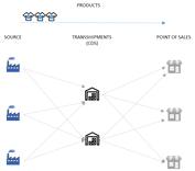
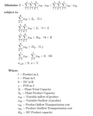
Let’s start by presenting a very traditional supply chain design problem as the multiple-commodity transshipment problem.
In this problem, you minimize the total cost of fulfilling the demand for a set of products at each point of sales, while sharing capacity constraints on plants and distribution centers.
Data
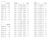
For this problem, we have a template-ready dataset from a spreadsheet, this will have the following structure:
- Node: Set of each entity of the model with their names
- Flow cost: The cost related to sending each product to plant x DC and DC x region
- Capacity: The total capacity of the Plants and DCs
- Node Arcs: The demand per region/product and capacity of production of each plant/product
path <- "Transshipment_template.xlsx"

data <- path %>%
  readxl::excel_sheets() %>%
  purrr::set_names() %>%
  purrr::map(readxl::read_excel, path = path)
To run the model, we must set it to the appropriate structure of R for optimization, this requires a set of data wrangling:
transship_wrang <- function(data){

  Product <- dplyr::filter(data$Nodes, Entity == "Product")$Name
  Plant <-  dplyr::filter(data$Nodes, Entity == "Plant")$Name
  DC <-  dplyr::filter(data$Nodes, Entity == "DC")$Name
  Region <-  dplyr::filter(data$Nodes, Entity == "Region")$Name

  incost <- dplyr::filter(data$flow_cost, type == "inflow")

  incst <- array(
	as.matrix(incost$value),
	dim = c(length(Product), length(Plant), length(DC)),
	dimnames = list(Product, Plant, DC)
  )

  outcost <- dplyr::filter(data$flow_cost, type == "outflow")

  outcst <- array(
	as.matrix(outcost$value),
	dim = c(length(Product), length(DC),length(Region)),
	dimnames = list(Product, DC, Region)
  )

  PlCapacity <- matrix(
	dplyr::filter(data$Capacity, Node == "Plant")$Value,
	ncol = 1,
	dimnames = list(Plant, "PlCapacity")
  )

  DCCapacity <- matrix(
	dplyr::filter(data$Capacity, Node == "DC")$Value,
	ncol = 1,
	dimnames = list(DC, "DCCapacity")
  )

  PlPrCapacity <- array(
	dplyr::filter(data$NodeARCs, Type == "Restriction")$Value,
	dim = c(length(Plant),length(Product)),
	dimnames = list(Plant, Product)
  )

  Demand <- array(
	dplyr::filter(data$NodeARCs, Type == "Demand")$Value,
	dim = c(length(Region),length(Product)),
	dimnames = list(Region, Product)
  )

  return(
	list(
  	Product = Product,
  	Plant = Plant,
  	DC = DC,
  	Region = Region,
  	incst = incst,
  	outcst = outcst,
  	PlPrCapacity = PlPrCapacity,
  	PlCapacity = PlCapacity,
  	DCCapacity = DCCapacity,
  	Demand = Demand
	)
  )
}

clean_data <- transship_wrang(data)
Modeling the transshipment problem in R
To set this model, we’ll use ompr since it relates to the mathematical formulation of MILP models, this eases the code x model barrier:
transship_model <- function(
	Product, Plant, DC, Region, incst, outcst,
	PlPrCapacity, PlCapacity, DCCapacity, Demand) {

  require(ROI)
  require(ROI.plugin.glpk)

  l <- length(Product) # Number of Products
  i <- length(Plant) #Number of Plants
  k <- length(DC) #Number of transhipments (CDs)
  j <- length(Region) #Number of cities (POS)

model <- ompr::MIPModel() %>%

  # Variable of inflow
  ompr::add_variable(xinf[l,i,k], l = 1:l, i = 1:i, k=1:k, type = "integer", lb = 0) %>%

  # Variable of outflow
  ompr::add_variable(xout[l,k,j], l = 1:l, k = 1:k, j=1:j, type = "integer", lb = 0) %>%

  ompr::set_objective(
	ompr::sum_expr(xinf[l,i,k] * incst[l,i,k], l = 1:l, i = 1:i, k=1:k) +  #Inbound Cost
	ompr::sum_expr(xout[l,k,j] * outcst[l,k,j], l = 1:l, k = 1:k, j=1:j) #Outbound Cost
  ) %>%

    #Plant Production Capacity
ompr::add_constraint(ompr::sum_expr(xinf[l,i,k], k=1:k) <= PlPrCapacity[i,l], l=1:l, i=1:i) %>%

  #Plant Total Capacity
  ompr::add_constraint(ompr::sum_expr(xinf[l,i,k], l=1:l, k=1:k) <= PlCapacity[i], i=1:i) %>%

  #DC Total Capacity
  ompr::add_constraint(ompr::sum_expr(xinf[l,i,k], l=1:l, i=1:i) <= DCCapacity[k], k=1:k) %>%

  #Fulfill Demand
  ompr::add_constraint(ompr::sum_expr(xout[l,k,j], k=1:k) >= Demand[j,l], l=1:l, j=1:j) %>%

  #Flow Constraint
  ompr::add_constraint(
    ompr::sum_expr(xinf[l,i,k], i=1:i) == ompr::sum_expr(xout[l,k,j], j=1:j),
    l=1:l, k=1:k
  )

  #Solve
  result <- ompr::solve_model(model, ompr.roi::with_ROI(solver = "glpk"))

  # Results

  objective <- result$objective_value

 Infl <- ompr::get_solution(result, xinf[l,i,k]) %>%
    dplyr::mutate(product = Product[l], source = Plant[i], destiny = DC[k], type = "Inflow") %>%
    dplyr::select(type, product, source, destiny, value)

 Outfl <- ompr::get_solution(result, xout[l,k,j]) %>%
  dplyr::mutate(product = Product[l], source = DC[k], destiny = Region[j], type = "Outflow") %>%
   dplyr::select(type, product, source, destiny, value)

  Dcs_Flow <- Infl %>%
	dplyr::group_by(destiny, product) %>%
	dplyr::summarise(Amount = sum(value)) %>%
	as.data.frame()

  Plants_Product <- Infl %>%
	dplyr::group_by(source, product) %>%
	dplyr::summarise(Amount = sum(value)) %>%
	as.data.frame()

  Products_flow <- rbind(Infl, Outfl)

  return(
	list(
  	objective = objective,
  	inflow = Infl,
  	outflow = Outfl,
  	Products_flow = Products_flow,
  	Dcs_Flow = Dcs_Flow,
  	Plants_Product = Plants_Product
	)
  )
}

model <- transship_model(
  Product = clean_data$Product,
  Plant = clean_data$Plant,
  DC = clean_data$DC,
  Region = clean_data$Region,
  incst = clean_data$incst,
  outcst = clean_data$outcst,
  PlPrCapacity = clean_data$PlPrCapacity,
  PlCapacity = clean_data$PlCapacity,
  DCCapacity = clean_data$DCCapacity,
  Demand = clean_data$Demand
)
Results
bootstrap <- c("striped", "hover", "responsive") glue::glue("Total Cost: {model$objective}") knitr::kable(model$Plants_Product, caption = "Plants Production") %>%
  kableExtra::kable_styling(bootstrap_options = bootstrap, full_width = F, font_size = 20, position = "float_left")

knitr::kable(model$Dcs_Flow, caption = "DCs Flow") %>%
  kableExtra::kable_styling(bootstrap_options = bootstrap, full_width = F, font_size = 20, position = "right")

knitr::kable(model$inflow, caption = "Inflow") %>%
  kableExtra::kable_styling(bootstrap_options = bootstrap, full_width = F, font_size = 20, position = "float_left")

knitr::kable(model$outflow, caption = "Outflow") %>%
  kableExtra::kable_styling(bootstrap_options = bootstrap, full_width = F, font_size = 20, position = "right")
Total Cost: 9250
Sharing SCM results using R Shiny
You and your team developed a great model and now have valuable insight for the company. How do you share this info with your peers? And can you make this insight interactive, letting them tweak values or set new input data?
You can do this and more by using R Shiny – an interactive web framework for R (and Python).
Are you more of a Python fan? See what’s currently possible with our Shiny for Python demo.
Continue below for the full code to build your own Shiny application for your SCM model.
Aesthetic functions
sankey_chart <- function(data, product) { data %>%
    dplyr::filter(product == !!product) %>%
    echarts4r::e_charts() %>%
    echarts4r::e_sankey(source, destiny, value) %>%
    echarts4r::e_title(glue::glue("Product {product} flow")) %>%
    echarts4r::e_tooltip() %>%
    echarts4r::e_theme("dark")
}

reactablefmtr <- function(data, args = TRUE, ...) { data %>%
    dplyr::select(...) %>%
    reactable::reactable(.,
      filterable = args, searchable = args, resizable = args,
      onClick = "select", outlined = TRUE, bordered = TRUE, borderless = TRUE,
      striped = args, highlight = TRUE, compact = args, showSortable = TRUE,
      theme = reactablefmtr::slate()
    )
}
Shiny UI
ui <- bs4Dash::dashboardPage(
 ui <- bs4Dash::dashboardPage(
  title = "Trasshipment Model",
  fullscreen = TRUE,
  dark = T,
  scrollToTop = T,
  header = bs4Dash::dashboardHeader(
    status = "gray-dark",
    title = bs4Dash::dashboardBrand(
      title = "Transshipment Model",
      color = "primary"
    )
  ),
  sidebar = bs4Dash::dashboardSidebar(
    collapsed = T,
    bs4Dash::sidebarMenu(
      bs4Dash::menuItem(
        text = "Transshipment",
        tabName = "transshipment",
        icon = icon("project-diagram")
      )
    )
  ),
  footer = bs4Dash::dashboardFooter(
    right = a(
      href = "https://appsilon.com/",
      "Built with ❤ by Appsilon"
    ),
    left = div(
      icon("calendar"),
      Sys.Date()
    ),
    fixed = T
  ),
  body = bs4Dash::dashboardBody(
    bs4Dash::tabItems(
      bs4Dash::tabItem(
        tabName = "transshipment",
        bs4Dash::tabBox(
          width = 12,
          collapsible = FALSE,
          maximizable = TRUE,
          tabPanel(
            "Model",
            fluidRow(
              column(
                4,
                bs4Dash::box(
                  status = "purple",
                  collapsible = F,
                  width = 12,
                  div(
                    class = "d-flex justify-content-center",
                    a(
                      tags$i(class = "fa fa-database"),
                      href = "www/files/Transshipment_template.xlsx",
                      "Download template",
                      class = "btn btn-default m-1",
                      download = NA, target = "_blank"
                    )
                  ),
                  hr(),
                  fileInput("uploadmodel", "Upload Data"),
                  hr(),
                  div(
                    class = "d-flex justify-content-center",
                    shiny::actionButton(
                      inputId = "model_run",
                      class = "btn btn-success action-button m-1 shiny-bound-input",
                      icon = icon("magic"),
                      label = "Run Model"
                    )
                  )
                )
              ),
              column(
                8,
                bs4Dash::tabBox(
                  width = 12,
                  collapsible = T,
                  maximizable = T,
                  collapsed = F,
                  tabPanel(
                    "Model Info",
                    div(
                      fluidRow(
                        bs4Dash::bs4ValueBoxOutput("products", width = 3),
                        bs4Dash::bs4ValueBoxOutput("plants", width = 3),
                        bs4Dash::bs4ValueBoxOutput("dcs", width = 3),
                        bs4Dash::bs4ValueBoxOutput("regions", width = 3)
                      ),
                      hr(),
                      selectInput(
                        "url_db",
                        label = h5("Choose the data"),
                        choices = c("Nodes", "flow_cost", "Capacity", "NodeARCs")
                      ),
                      shinycssloaders::withSpinner(
                        reactable::reactableOutput("data"),
                        type = 8
                      )
                    )
                  ),
                  tabPanel(
                    "Results",
                    uiOutput("ui_output")
                  )
                )
              )
            )
          )
        )
      )
    )
  )
)
Server – Deploying your Supply Chain Management Shiny app
server <- function(input, output) {
  data <- reactive({
    path <- input$uploadmodel$datapath path %>%
      readxl::excel_sheets() %>%
      purrr::set_names() %>%
      purrr::map(readxl::read_excel, path = path)
  })

  data_info <- reactive(
    transship_wrang(data())
  )

  output$products <- bs4Dash::renderbs4ValueBox({
    req(input$uploadmodel$datapath)
    bs4Dash::bs4ValueBox(length(data_info()$Product), subtitle = "Products", color = "primary")
  })

  output$plants <- bs4Dash::renderbs4ValueBox({
    req(input$uploadmodel$datapath)
    bs4Dash::bs4ValueBox(length(data_info()$Plant), subtitle = "Plants", color = "primary")
  })

  output$dcs <- bs4Dash::renderbs4ValueBox({
    req(input$uploadmodel$datapath)
    bs4Dash::bs4ValueBox(length(data_info()$DC), subtitle = "DCs", color = "primary")
  })

  output$regions <- bs4Dash::renderbs4ValueBox({
    req(input$uploadmodel$datapath)
    bs4Dash::bs4ValueBox(length(data_info()$Region), subtitle = "Regions", color = "primary")
  })

  output$data <- reactable::renderReactable({
    req(input$uploadmodel$datapath)
    reactablefmtr(data()[input$url_db][[1]], args = FALSE, everything())
  })

  observeEvent(input$model_run, {

    if (is.null(input$uploadmodel$datapath)) {
      shinyWidgets::sendSweetAlert(
        title = "Upload a file",
        type = "error",
        text = "Please, Upload a file first"
      )
    } else {
      model <- transship_model(
          Product = data_info()$Product,
          Plant = data_info()$Plant,
          DC = data_info()$DC,
          Region = data_info()$Region,
          incst = data_info()$incst,
          outcst = data_info()$outcst,
          PlPrCapacity = data_info()$PlPrCapacity,
          PlCapacity = data_info()$PlCapacity,
          DCCapacity = data_info()$DCCapacity,
          Demand = data_info()$Demand
        )

      output$total_value <- renderText({
        glue::glue("Total Cost: {model$objective}")
      })

      output$sankey_chart <- echarts4r::renderEcharts4r({
        sankey_chart(model$Products_flow, input$product)
      })

      output$results_data <- reactable::renderReactable({
        reactablefmtr(model[input$result_data][[1]], args = FALSE, everything())
      })

      output$ui_output <- renderUI({

        tagList(
          div(
            class = "d-flex justify-content-center",
            h2(textOutput("total_value"))
          ),
          selectInput(
            "product",
            label = h5("Choose Product"),
            choices = data_info()$Product
          ),
          echarts4r::echarts4rOutput("sankey_chart"),
          selectInput(
            "result_data",
            label = h5("Choose view"),
            choices = c("inflow", "outflow", "Dcs_Flow", "Plants_Product")
          ),
          reactable::reactableOutput("results_data")
        )
      })
    }
  })
}
Running the application
shinyApp(ui = ui, server = server)
Summing up R and Shiny in Supply Chain Management
Supply chain management has many layers of solutions and models designed for each scope of the business strategy. The intrinsic trade-off between those strategies requires visibility, and by being reproducible, R is capable of delivering value to each step in the strategy spectrum.
There are solutions where a spreadsheet definitely shines, especially while designing an idea from scratch. But with R you can extend this to a business-friendly solution in a production-ready state without compromising the flexibility you require for your business life cycle.
There are many other topics in supply chain and applications that can be used with R, but the main insight for this post is that reproducibility is a key factor for success in the alignment between the scope of strategies. This is vital for businesses and makes a significant difference in sustainable and successful solutions.
And as your project grows, you can scale R Shiny and add greater business value using enterprise solutions like RStudio products.
