

R Data Processing Frameworks: How To Speed Up Your Data Processing Pipelines up to 20 Times
Picture this – the data science team you manage primarily uses R and heavily relies on dplyr for implementing data processing pipelines. All is good, but then out of the blue you’re working with a client that has a massive dataset, and all of a sudden dplyr becomes the bottleneck. You want a faster way to process data with minimum to no changes to the source code.
You’re wondering, how much effort will it take to speed up your data processing pipelines 2 times, 5 times, 10 times, or even up to 20 times? The answer might surprise you – far less than you think.
This article will show you why dplyr fails to perform on larger datasets, and which alternative options you have in the context of R data processing frameworks. Let’s dig in!
R is full of things you didn’t know are possible – Here’s a couple of advanced Excel functions in R for data manipulation.
Table of contents:
- Dplyr Alternatives – Top R Data Processing Frameworks
- Dplyr vs. Arrow vs. DuckDB – R Data Processing Framework Test
- Summing up R Data Processing Framework Benchmarks
Dplyr Alternatives – Top R Data Processing Frameworks
This section will introduce you to two dplyr alternatives that use the same interface – arrow and duckdb. We wanted to focus on these two specifically because they come up with minimal code changes, as you’ll see from the examples later. They provide the best “bang for the buck” if your data science team doesn’t have the time to learn a new data processing framework from scratch.
Which R dplyr Alternatives Can You Use?
Sure, everyone loves dplyr. We’ve even dedicated a full article for beginner-level data analysis techniques with dplyr. The package has a user-friendly syntax and is super easy to use for data transformation tasks. But guess what – so are the other two alternatives we’ll use today. In addition, they are usually up to 20 times faster.
Arrow is a cross-language development platform for in-memory and larger-than-memory data. The R package exposes an interface to the Arrow C++ library, allowing you to benefit from an R programming language syntax, and access to a C++ library API through a set of well-known dplyr backend functions. Arrow also provides zero-copy data sharing between R and Python, which might be appealing for language-agnostic data science teams.
You can learn more about Arrow for R here.
DuckDB is an open-source, embedded, in-process, relational OLAP DBMS. Its description contains pretty much every buzzword you could imagine, but it being an OLAP database means the data is organized by columns and is optimized for complex data queries (think joins, aggregations, groupings, and so on). The good thing about duckdb is that it comes with an R API, meaning you can use R to point to a local (or remote) instance of your database with DBI. Further, duckdb R package uses dplyr-like syntax, which means code changes coming from a vanilla dplyr will be minimal to non-existent.
You can learn more about DuckDB here and about its R API here.
So, these are the dplyr alternatives we’ll use to perform a series of benchmarks with the goal of comparing R data processing frameworks. They should both be faster than dplyr in most cases, but that’s where the actual tests come in. More on that in the following section.
Dplyr vs. Arrow vs. DuckDB – R Data Processing Framework Test
To kick things off, let’s talk about data. We have several small to somewhat large Parquet files and a single DuckDB database (not publicly available) that has other files stored inside. The dplyr and arrow benchmarks will be based on the Parquet files, and the DuckDB benchmarks will be connected to the local database:
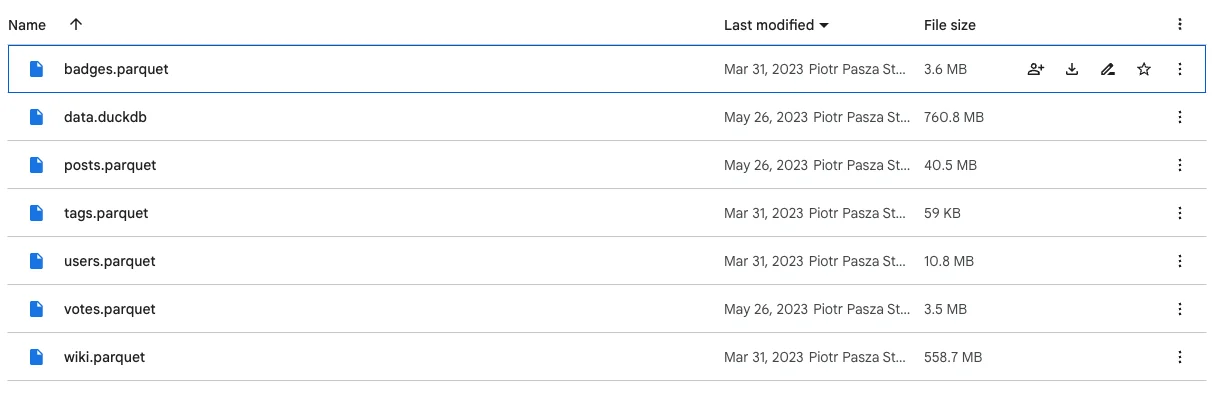
Image 1 – Datasets used
Next, we’ll discuss how the benchmarks were configured, R package versions, and the hardware used to run the tests.
Benchmark Setup and Information
As for R itself, we’ve used R version 4.3.1. The most important packages were installed with the following version numbers:
dplyr– 1.1.3arrow– 13.0.0duckdb– 0.8.1-3
Each of the benchmark tests you’ll see below was run 3 times for each R data processing framework.
The hardware of choice was a 14″ M2 Pro MacBook Pro with a 12-core CPU and 16 GB of RAM.
For working on dplyr and arrow benchmarks, we’ve imported the following R packages:
library(tidyverse)
library(arrow)
The arrow benchmark results have had the following option configured:
options(arrow.pull_as_vector = TRUE)Working with duckdb required a couple of extra dependencies:
library(DBI)
library(duckdb)
In both of these, the following code was used to load the datasets:
badges <- read_parquet("../../data/badges.parquet")
posts <- read_parquet("../../data/posts.parquet")
tags <- read_parquet("../../data/tags.parquet")
users <- read_parquet("../../data/users.parquet")
votes <- read_parquet("../../data/votes.parquet")
wiki <- read_parquet("../../data/wiki.parquet")
In order to connect to a DuckDB database and extract the datasets, we’ve used the following code:
con <- dbConnect(duckdb::duckdb("./data.duckdb"))

badges <- tbl(con, "badges")
posts <- tbl(con, "posts")
tags <- tbl(con, "tags")
users <- tbl(con, "users")
votes <- tbl(con, "votes")
wiki <- tbl(con, "wiki")
Finally, to actually run benchmarks, we decided to declare a benchmark() function which takes another function as an argument:
benchmark <- function(fun) {
    start <- Sys.time()
    res <- fun()
    end <- Sys.time()
    print(end - start)
    res
}
Each of the 8 benchmarks you’ll see below wraps the logic inside a separate function and then calls benchmark() and passes itself as an argument.
So with that out of the way, let’s go over our first benchmark!
Benchmark #1: Finding the Article with the Most External Entries
The goal of the first benchmark was to use the wiki dataset to find the article with the most external entries on English Wikipedia in March 2022.
You’ll find the code for all three R packages below. The only difference from vanilla dplyr is in passing some additional arguments to summarise() and slice_max() functions. Everything else is identical:
b1_dplyr <- function() {
  wiki %>%
    filter(type == "external") %>%
    group_by(curr) %>%
    summarise(total = sum(n)) %>%
    slice_max(total, n = 3) %>%
    pull(curr)
}

b1_arrow <- function() {
  wiki %>%
    filter(type == "external") %>%
    group_by(curr) %>%
    summarise(total = sum(n)) %>%
    slice_max(total, n = 3, with_ties = FALSE) %>%
    pull(curr)
}

b1_duckdb <- function() {
  wiki %>%
    filter(type == "external") %>%
    group_by(curr) %>%
    summarise(total = sum(n, na.rm = TRUE)) %>%
    slice_max(total, n = 3, with_ties = FALSE) %>%
    pull(curr)
}
Here are the results:
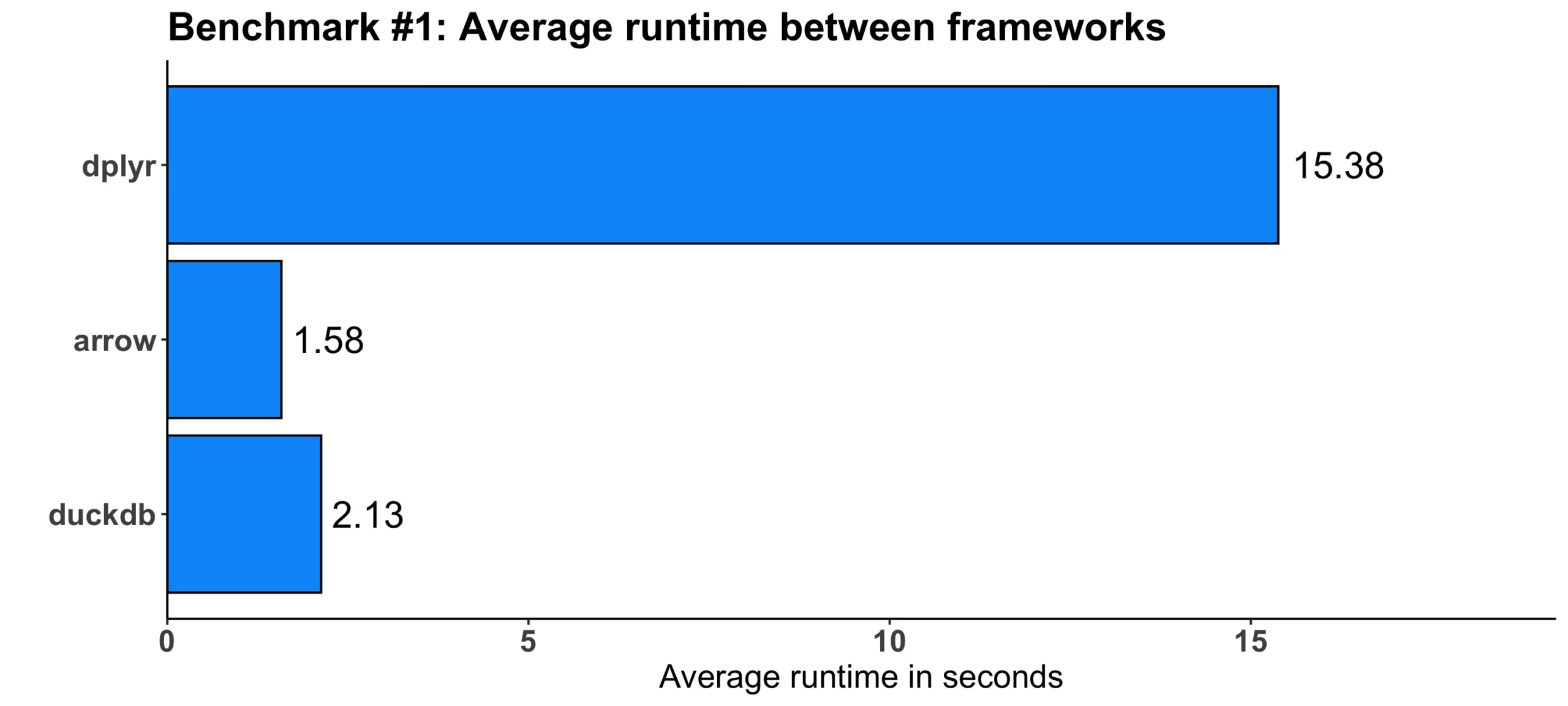
Image 2 – Benchmark #1 results
As you can see, both arrow and duckdb were faster, by 10 and 7 times, respectively.
Benchmark #2: Finding Properties Across Multiple Datasets
The second test was a combination of two calculations – the first one had the task of finding the DisplayName property of a user that has the most badges, while the second one had to find the Location property for the same condition. Most of the logic is implemented in the first portion of the calculation, where the ID of the user was found, and then in the second portion, only the desired properties were extracted.
As before, most of the code differences boil down to the extra arguments in a couple of functions and calling collect() at the end of the calculation:
b2_dplyr <- function() {
  tid <- badges %>%
    left_join(users, by = join_by(UserId == Id)) %>%
    group_by(UserId, DisplayName) %>%
    summarise(NBadges = n()) %>%
    ungroup() %>%
    slice_max(NBadges, n = 1) %>%
    pull(UserId)
  top_user <- users %>%
    filter(Id == tid) %>%
    select(DisplayName, Location)

  top_user
}


b2_arrow <- function() {
  tid <- badges %>%
    left_join(users, by = join_by(UserId == Id)) %>%
    group_by(UserId, DisplayName) %>%
    summarise(NBadges = n()) %>%
    ungroup() %>%
    slice_max(NBadges, n = 1, with_ties = FALSE) %>%
    pull(UserId)

  top_user <- users %>%
    filter(Id == tid) %>%
    select(DisplayName, Location)

  top_user %>% collect()
}


b2_duckdb <- function() {
  tid <- badges %>%
    left_join(users, by = join_by(UserId == Id)) %>%
    group_by(UserId, DisplayName) %>%
    summarise(NBadges = n()) %>%
    ungroup() %>%
    slice_max(NBadges, n = 1, with_ties = FALSE) %>%
    pull(UserId)

  top_user <- users %>%
    filter(Id == tid) %>%
    select(DisplayName, Location)

  top_user %>% collect()
}
These are the results we got:
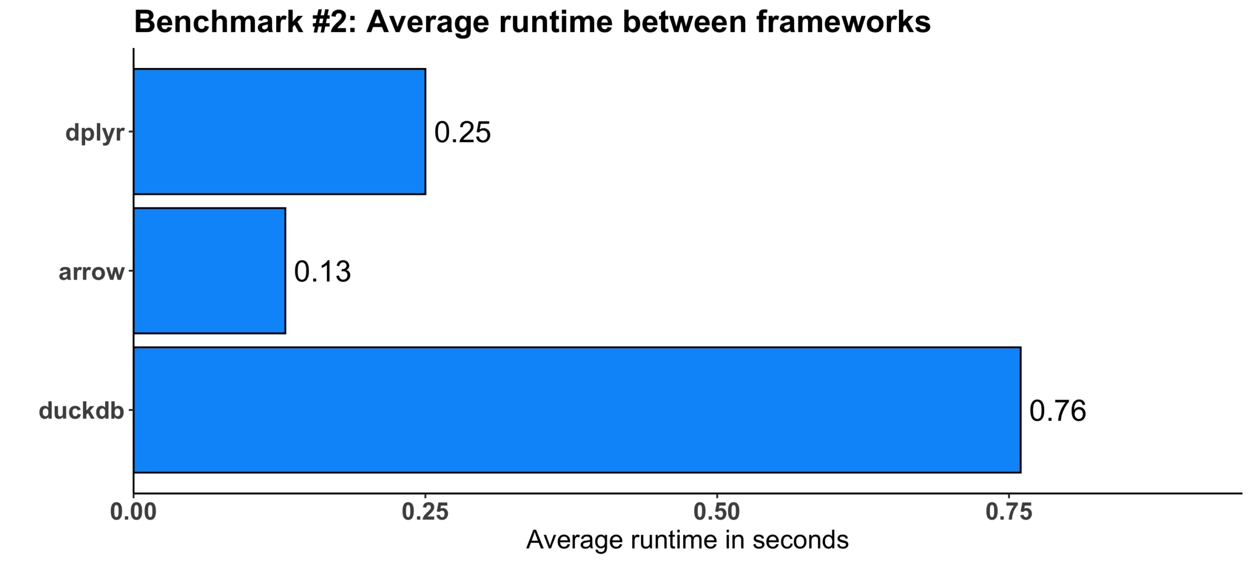
Image 3 – Benchmark #2 results
The truth is – dplyr wasn’t the slowest one here. arrow was still almost twice as fast, but duckdb was three times slower on average.
Benchmark #3: Finding the Number of Entries
The third test used the wiki dataset to find the number of entries on the article about the city from the previous benchmark on English Wikipedia in March 2022.
Both dplyr alternatives introduce the collect() method at the end of the calculation and also some additional arguments to the summarise() function:
b3_dplyr <- function() {
  city <- str_split(top_user %>% pull(Location), ",")[[1]][[1]]
  wiki %>%
    filter(curr == city) %>%
    summarise(sum(n))
}

br_arrow <- function() {
  city <- str_split(top_user %>% pull(Location), ",")[[1]][[1]]
  wiki %>%
    filter(curr == city) %>%
    summarise(sum(n)) %>%
    collect()
}

b3_duckdb <- function() {
  city <- str_split(top_user %>% pull(Location), ",")[[1]][[1]]
  wiki %>%
    filter(curr == city) %>%
    summarise(sum(n, na.rm = TRUE)) %>%
    collect()
}
Here’s what we got out of the tests:
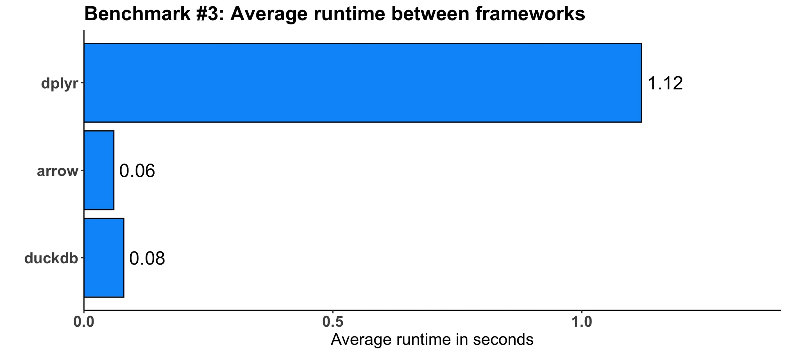
Image 4 – Benchmark #3 results
In absolute terms, the difference isn’t that large, but speaking relatively, arrow proved to be around 18 times faster, while duckdb was 14 times faster. Impressive!
Benchmark #4: Finding the Most Common Words with a Given Condition
The fourth test was once again a combination of two aggregations, one on the posts dataset, and the other on wiki dataset. The first one had the task of finding the most common work with at least 8 characters. The second one then found the number of occurrences of the most common word with at least 8 characters in all posts.
This is where we see a couple of significant syntax differences among different R data processing frameworks. The dplyr package requires you to write the least amount of code, as you can see below:
b4_dplyr <- function() {
  theword <- posts %>%
    select(Body) %>%
    mutate(Body = gsub("<.*?>", "", Body)) %>%
    mutate(Body = gsub("\n", " ", Body)) %>%
    separate_rows(Body, sep = " ") %>%
    rename(Words = Body) %>%
    filter(nchar(Words) > 7) %>%
    count(Words) %>%
    slice_max(n, n = 1) %>%
    pull(Words)

  sum_of_n <- wiki %>%
    filter(curr == str_to_title(theword)) %>%
    summarize(sum_n = sum(n)) %>%
    pull()
  paste(theword, sum_of_n)
}

b4_arrow <- function() {
  theword <- posts %>%
    select(Body) %>%
    mutate(Body = gsub("<.*?>", "", Body)) %>%
    mutate(Body = gsub("\n", " ", Body)) %>%
    collect() %>%
    separate_rows(Body, sep = " ") %>%
    as_arrow_table() %>%
    rename(Words = Body) %>%
    filter(nchar(Words) > 7) %>%
    count(Words) %>%
    slice_max(n, n = 1, with_ties = FALSE) %>%
    pull(Words)

  sum_of_n <- wiki %>%
    filter(curr == str_to_title(theword)) %>%
    summarize(sum_n = sum(n)) %>%
    pull()

  paste(theword, sum_of_n)
}

b4_duckdb <- function() {
  theword <- posts %>%
    select(Body) %>%
    mutate(Body = regexp_replace(Body, "<.*?>", "", "g")) %>%
    mutate(Body = regexp_replace(Body, "\n", " ")) %>%
    mutate(Body = string_split(Body, " ")) %>%
    mutate(Body = unnest(Body)) %>%
    mutate(Body = lower(Body)) %>%
    rename(Words = Body) %>%
    filter(nchar(Words) > 7) %>%
    count(Words) %>%
    slice_max(n, n = 1, with_ties = FALSE) %>%
    pull(Words)
  theword <- str_to_title(theword)
  sum_of_n <- wiki %>%
    filter(curr == theword) %>%
    summarize(sum_n = sum(n, na.rm = TRUE)) %>%
    pull()

  paste(theword, sum_of_n)
}
But at what cost? Let’s examine the benchmark results next:
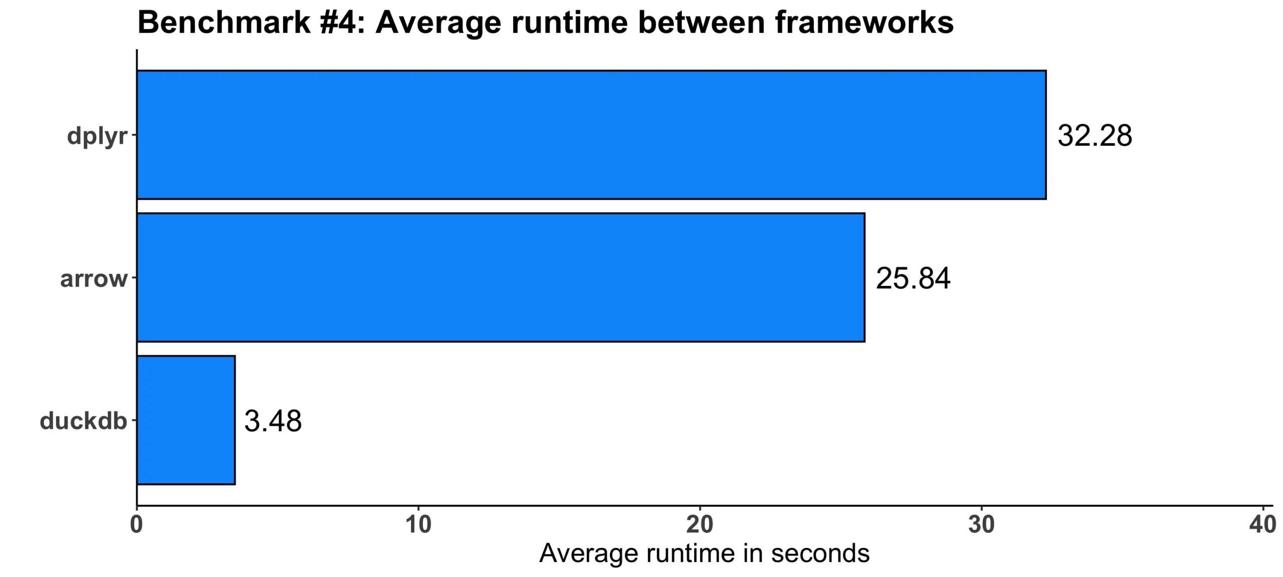
Image 5 – Benchmark #4 results
This time, duckdb was a clear winner, outperforming dplyr by a factor of 9. arrow was only slightly faster than dplyr, by around 6 and a half seconds or 25%.
Benchmark #5: Finding the Largest Difference in Multiple Datasets
This test used the votes and posts datasets to first find the post with the highest difference between upvotes and downvotes, and then find the DisplayName property along with the actual difference between upvotes and downvotes. It’s a lot to take in at once, but most of it boils down to running multiple computations sequentially, and there aren’t many code differences between our three data processing frameworks.
Feel free to take a look at the code and decide by yourself:
b5_dplyr <- function() {
  upvotes <- votes %>%
    filter(VoteTypeId == 2) %>%
    group_by(PostId) %>%
    summarize(UpVotes = n()) %>%
    ungroup()

  downvotes <- votes %>%
    filter(VoteTypeId == 3) %>%
    group_by(PostId) %>%
    summarize(DownVotes = n()) %>%
    ungroup()

  posts2 <- posts %>%
    left_join(upvotes, by = c("Id" = "PostId")) %>%
    left_join(downvotes, by = c("Id" = "PostId")) %>%
    mutate(
      UpVotes = coalesce(UpVotes, 0),
      DownVotes = coalesce(DownVotes, 0)
    ) %>%
    mutate(UpVoteRatio = UpVotes - DownVotes)

  posts2 %>%
    inner_join(users, by = c("OwnerUserId" = "Id")) %>%
    arrange(desc(UpVoteRatio)) %>%
    slice(1) %>%
    select(Score, DisplayName)
}

b5_arrow <- function() {
  upvotes <- votes %>%
    filter(VoteTypeId == 2) %>%
    group_by(PostId) %>%
    summarize(UpVotes = n()) %>%
    ungroup()

  downvotes <- votes %>%
    filter(VoteTypeId == 3) %>%
    group_by(PostId) %>%
    summarize(DownVotes = n()) %>%
    ungroup()

  posts2 <- posts %>%
    left_join(upvotes, by = c("Id" = "PostId")) %>%
    left_join(downvotes, by = c("Id" = "PostId")) %>%
    mutate(
      UpVotes = coalesce(UpVotes, 0),
      DownVotes = coalesce(DownVotes, 0)
    ) %>%
    mutate(UpVoteRatio = UpVotes - DownVotes)

  posts2 %>%
    inner_join(users, by = c("OwnerUserId" = "Id")) %>%
    slice_max(UpVoteRatio, n = 1, with_ties = FALSE) %>%
    select(Score, DisplayName) %>%
    collect()
}

b5_duckdb <- function() {
  upvotes <- votes %>%
    filter(VoteTypeId == 2) %>%
    group_by(PostId) %>%
    summarize(UpVotes = n()) %>%
    ungroup()

  downvotes <- votes %>%
    filter(VoteTypeId == 3) %>%
    group_by(PostId) %>%
    summarize(DownVotes = n()) %>%
    ungroup()

  posts2 <- posts %>%
    left_join(upvotes, by = c("Id" = "PostId")) %>%
    left_join(downvotes, by = c("Id" = "PostId")) %>%
    mutate(
      UpVotes = coalesce(UpVotes, 0),
      DownVotes = coalesce(DownVotes, 0)
    ) %>%
    mutate(UpVoteRatio = UpVotes - DownVotes)

  posts2 %>%
    inner_join(users, by = c("OwnerUserId" = "Id")) %>%
    slice_max(UpVoteRatio, n = 1, with_ties = FALSE) %>%
    select(Score, DisplayName) %>%
    collect()
}
This is what we got in the end:
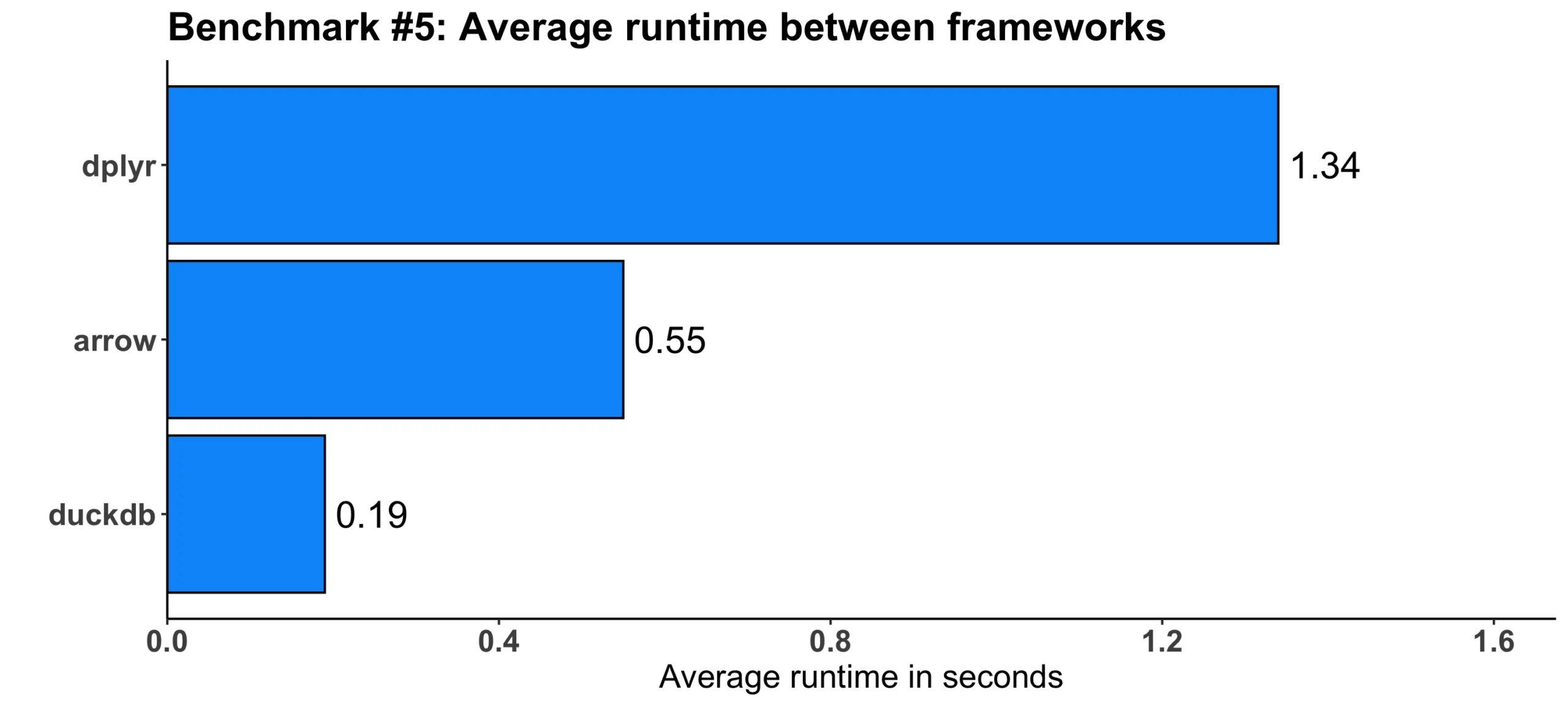
Image 6 – Benchmark #5 results
Once again, there is not a huge difference in absolute terms. But relatively speaking, arrow was 2.5 faster and duckdb was 7 times faster when compared to dplyr.
Benchmark #6: Finding the Month with the Most Posts Created
Our next test has a simple task of finding the month in which the most posts were created. That’s it!
The code differences are almost negligible here – both arrow and duckdb call the collect() method at the end and the order of operation is somewhat different between all three. Nothing you couldn’t change for yourself in a couple of minutes:
b6_dplyr <- function() {
  votes %>%
    mutate(CreationDateDT = as.POSIXct(CreationDate)) %>%
    arrange(CreationDateDT) %>%
    group_by(Month = floor_date(CreationDateDT, "month")) %>%
    summarize(Count = n()) %>%
    slice_max(Count, n = 1)
}

b6_arrow <- function() {
  votes %>%
    arrange(CreationDate) %>%
    collect() %>% # seems to be some bug that requires this
    group_by(Month = floor_date(CreationDate, "month")) %>%
    summarize(Count = n()) %>%
    slice_max(Count, n = 1, with_ties = FALSE) %>%
    collect()
}

b6_duckdb <- function() {
  votes %>%
    group_by(Month = floor_date(CreationDate, "month")) %>%
    summarize(Count = n()) %>%
    slice_max(Count, n = 1) %>%
    collect()
}
Here’s the outcome:
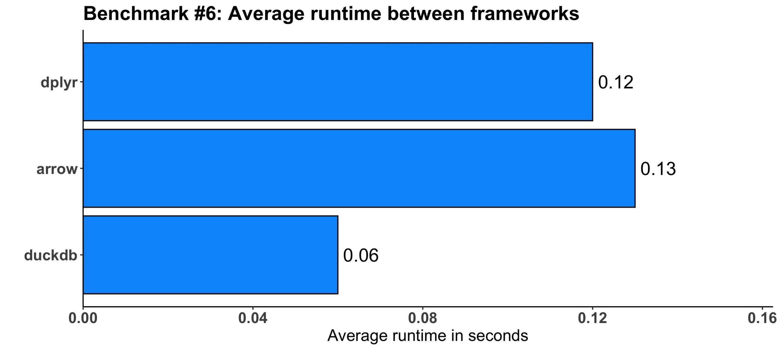
Image 7 – Benchmark #6 results
duckdb seems to be twice as fast on average when compared to dplyr. On the other hand, arrow was slower on average by a hundredth of a second.
Benchmark #7: Finding the Month with the Biggest Decrease in the Amount of Posts
The goal of our next test was to find the month in which there was the biggest decrease in the amount of created posts. Simple and straightforward, just like with the previous one.
arrow was the most verbose framework in this test, requiring a couple of extra lines of code and calling the collect() function twice:
b7_dplyr <- function() {
  votes %>%
    mutate(CreationDateDT = as.POSIXct(CreationDate)) %>%
    group_by(Month = floor_date(CreationDateDT, "month")) %>%
    summarize(VoteCount = n(), .groups = "drop") %>%
    mutate(Diff = VoteCount - lag(VoteCount)) %>%
    select(Month, Diff) %>%
    slice_min(Diff, n = 1)
}

b7_arrow <- function() {
  votes %>%
    group_by(Month = floor_date(CreationDate, "month")) %>%
    summarize(VoteCount = n(), .groups = "drop") %>%
    collect() %>%
    mutate(Diff = VoteCount - lag(VoteCount)) %>% # lag not supported in arrow
    as_arrow_table() %>%
    arrange(Diff) %>%
    select(Month, Diff) %>%
    slice_head(n = 1) %>%
    collect()
}

b7_duckdb <- function() {
  votes %>%
    group_by(Month = floor_date(CreationDate, "month")) %>%
    summarize(VoteCount = n(), .groups = "drop") %>%
    mutate(Diff = VoteCount - lag(VoteCount)) %>%
    select(Month, Diff) %>%
    slice_min(Diff, n = 1) %>%
    collect()
}
This is what we got:
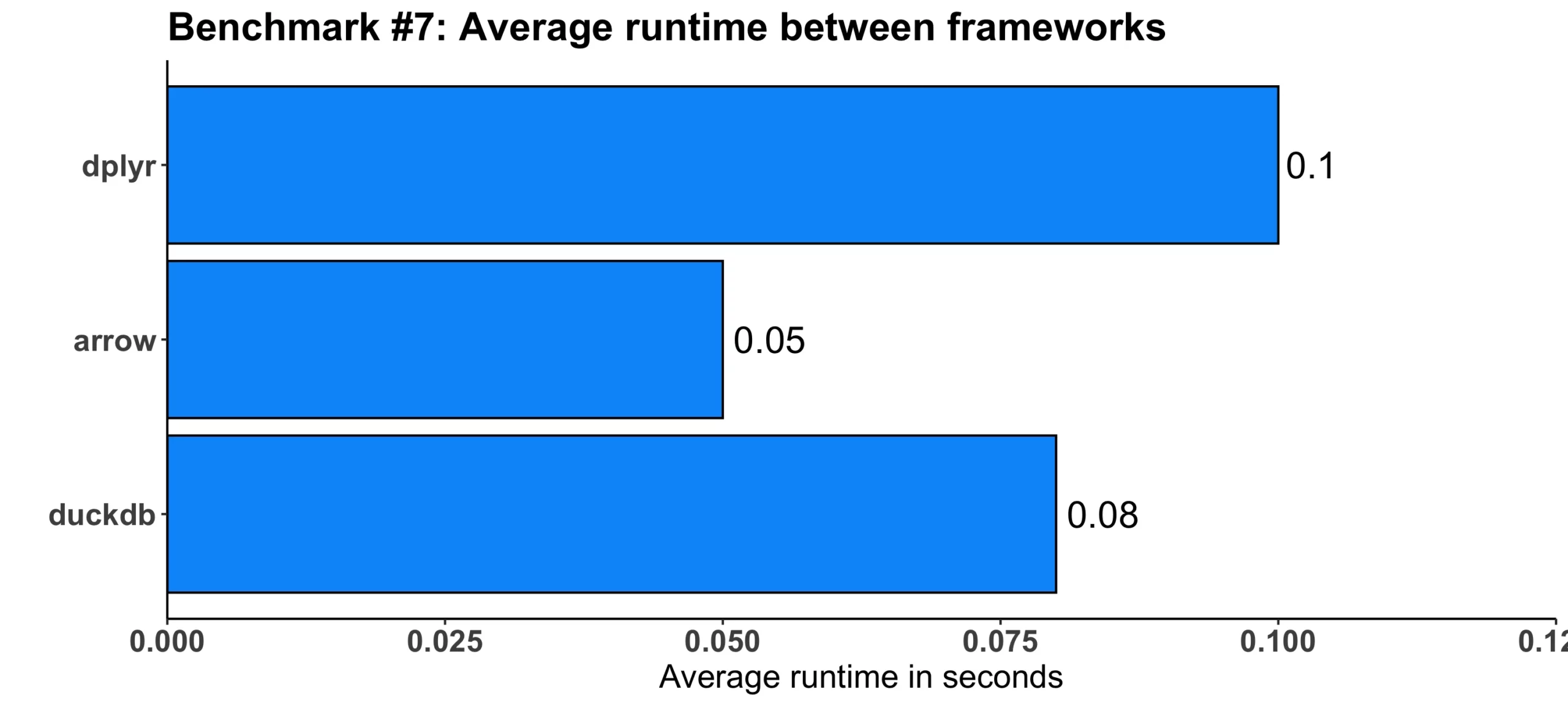
Image 8 – Benchmark #7 results
Despite the added verbosity, arrow was still twice faster than dplyr. The duckdb framework was somewhere in the middle, still having a slight edge over the vanilla dplyr.
Benchmark #8: Finding Common Tags Along Posts by Location
For the final test, the goal was to find the most common tag along posts created by users from Poland. To get this information, the Location column in the posts dataset should contain “Poland” or “Polska”.
The syntax is slightly different between our three data processing frameworks, with arrow being the most verbose one once again:
b8_dplyr <- function() {
  tags <- posts %>%
    left_join(users, by = c("OwnerUserId" = "Id")) %>%
    filter(str_detect(Location, "Poland|Polska")) %>%
    select(Tags) %>%
    mutate(Tags = str_replace_all(Tags, "[<>]", " ")) %>%
    separate_rows(Tags, sep = " ") %>%
    filter(Tags != "")

  tags %>%
    count(Tags) %>%
    arrange(desc(n)) %>%
    slice(1)
}

b8_arrow <- function() {
  tags <- posts %>%
    left_join(users, by = c("OwnerUserId" = "Id")) %>%
    filter(str_detect(Location, "Poland|Polska")) %>%
    select(Tags) %>%
    mutate(Tags = str_replace_all(Tags, "[<>]", " ")) %>%
    collect() %>%
    separate_rows(Tags, sep = " ") %>%
    as_arrow_table() %>%
    filter(Tags != "")

  tags %>%
    count(Tags) %>%
    slice_max(n, n = 1, with_ties = FALSE) %>%
    collect()
}

b8_duckdb <- function() {
  tags <- posts %>%
    left_join(users, by = c("OwnerUserId" = "Id")) %>%
    filter(str_detect(Location, "Poland|Polska")) %>%
    select(Tags) %>%
    mutate(Tags = str_replace_all(Tags, "[<>]", " ")) %>%
    mutate(Tags = string_split(Tags, " ")) %>%
    mutate(Tags = unnest(Tags)) %>%
    filter(Tags != "")

  tags %>%
    count(Tags) %>%
    slice_max(n, n = 1, with_ties = FALSE) %>%
    collect()
}
In the end, these are the time differences:
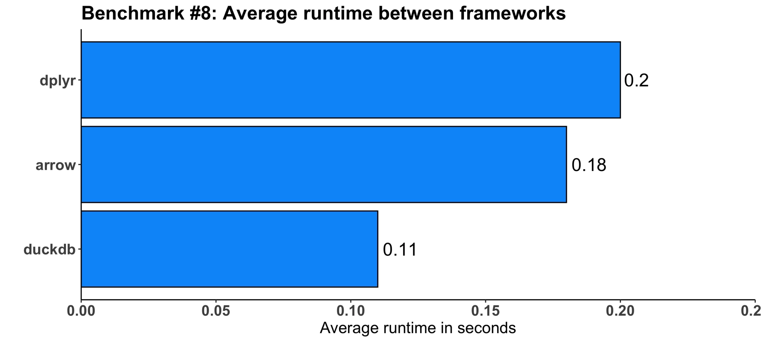
Image 9 – Benchmark #8 results
But this time, it was duckdb that was almost two times faster than dplyr. The arrow framework provided somewhat of a negligible 10% runtime decrease when compared to dplyr.
Conclusion: Which R Data Processing Framework Should You Use?
In the end, let’s imagine all of our 8 benchmarks make a single data processing pipeline. The question is – Which R data processing framework wins in total? Total here being the summation of average (of 3) runtimes for each benchmark.
Here are the results:
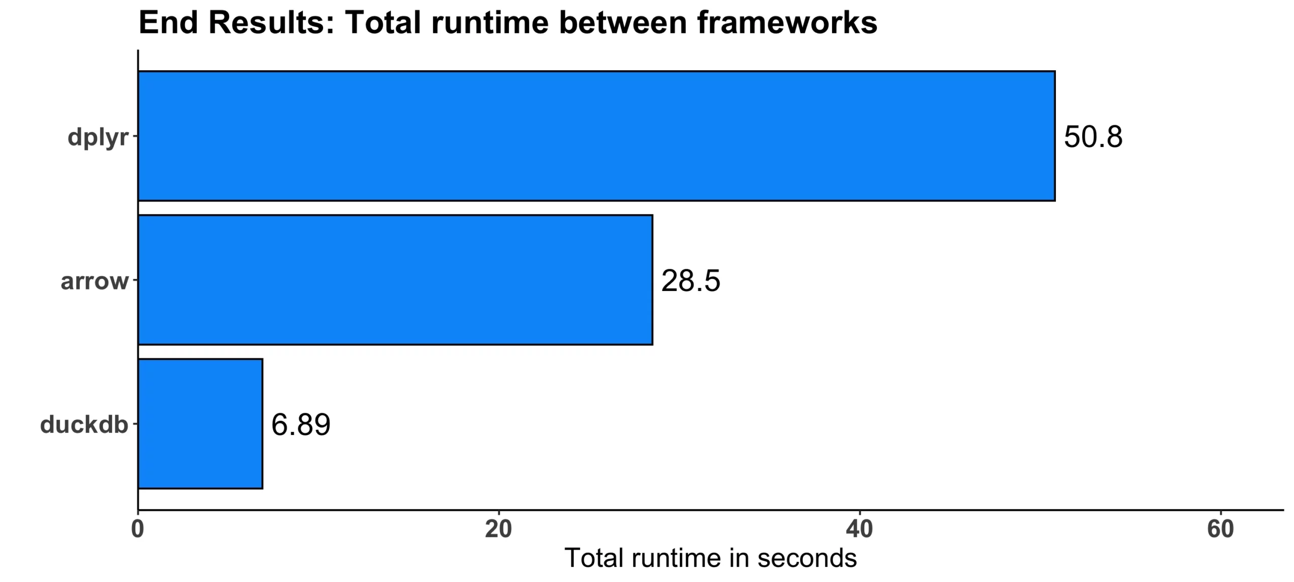
Image 10 – Total runtime comparison
It’s clear to say that duckdb won by a huge margin – it’s 7.4 times faster when compared to dplyr and 4.1 times faster when compared to arrow. This is mostly because of benchmark #4 results, in which duckdb won by 20-30 seconds in absolute terms.
Still, it makes sense to compare all three in your work environment to find out which data processing framework is the fastest for your specific needs. Now you know how, so you shouldn’t have any trouble cutting down the data processing runtime by a significant factor.
Summing up R Data Processing Framework Benchmarks
Long story short – it takes minimal effort (code changes) to massively speed up your data processing pipelines in R. The dplyr package is just fine when you’re just starting out, but you should look into the alternatives mentioned today when speed is of the essence. Spoiler alert, it always is.
But switching between R data processing frameworks doesn’t have to be a long an painful experience. Packages like arrow and duckdb use the same dplyr interface but provide much faster results. You can change the backend in a matter of minutes, or hours in a worst-case scenario if you have a lot of data processing pipelines.
What’s your go-to way of speeding up dplyr? Do you use the packages mentioned today or something else entirely? Make sure to let us know in the comment section below.
Looking to automate data quality reporting in R and R Shiny? Look no further than R’s data.validator package.

