R {targets}: How to Make Reproducible Pipelines for Data Science and Machine Learning

The R {targets} package is a pipeline tool for statistics, data science, and machine learning in R. The package allows you to write and maintain reproducible R workflows in pipelines that run only when necessary (e.g., either data or code has changed). The best part is – you’ll learn how to use it today.

By the end of the article, you’ll have an entire pipeline for loading, preparing, splitting, training and evaluating a logistic regression model on the famous Titanic dataset. You’ll see just how easy it is to use targets, and why it might be a good idea to use the package on your next data science project.

But what is Logistic Regression? Read our complete guide for machine learning beginners.

Table of contents:

• What Is R {targets} and Why Do You Need It?
• Let’s Code a Machine Learning Pipeline
• Machine Learning Pipeline in {targets} – Plain English Explanation
• Summing up R {targets}

What Is R {targets} and Why Do You Need It?

Data science and machine learning boil down to experimentation. Each experiment can take from seconds to days to complete, and by the end, the results might not be valid (if you update the code or the data).

That’s exactly the issue targets aims to solve. It enables you to maintain a reproducible workflow, learns how your pipeline fits together, skips the tasks that are already up to date, and runs only the necessary computations. This way, you save both time and compute power.

The package allows you to do your research and experiments entirely within R, which is a rare sight even in late 2022. Most pipeline tools are either language agnostic or Python-specific, so seeing something with native R support is always welcoming.

The projects in which you’ll use targets will have the following structure:

    ├── _targets.R
    ├── data.csv
    ├── R/
    │   ├── functions.R

The first file – _targets.R is created by the package, but more on that later. The data.csv serves as a dummy example of a data source. You don’t need it, as you can load data from a database or web instead. The only file you actually need is R/functions.R, as it will contain all the R functions that form your pipeline.

Create the folder and file if you haven’t already, and let’s start writing a couple of functions for training a machine learning model.

Let’s Code a Machine Learning Pipeline

As mentioned in the introduction section, we’ll write a machine learning pipeline for training and evaluating a logistic regression model on the Titanic dataset.

The pipeline will be spread over five R functions in R/functions.R file. Here’s a description of what each function does:

• get_data() – Returns the training subset of the Titanic dataset. We’ll use only this subset throughout the article.
• prepare_data() – A lengthy function that is used to clean up the dataset, extract meaningful features, drop unused ones, and impute missing values.
• train_test_split() – Splits our dataset into training and testing subsets (80:20).
• fit_model() – Fits a logistic regression model to the training set.
• evaluate_model() – Returns a confusion matrix of the test set.

It’s quite a long file, so feel free to just copy/paste it from the snippet below (don’t forget to install the packages if necessary):

library(titanic)
library(dplyr)
library(modeest)
library(mice)
library(caTools)
library(caret)

get_data <- function() {
  return(titanic_train)
}

prepare_data <- function(data) {
  # Convert empty strings to NaN
  data$Cabin[data$Cabin == ""] <- NA
  data$Embarked[data$Embarked == ""] <- NA

  # Title extraction
  data$Title <- gsub("(.*, )|(\\..*)", "", data$Name)
  rare_titles <- c("Dona", "Lady", "the Countess", "Capt", "Col", "Don", "Dr", "Major", "Rev", "Sir", "Jonkheer")
  data$Title[data$Title == "Mlle"] <- "Miss"
  data$Title[data$Title == "Ms"] <- "Miss"
  data$Title[data$Title == "Mme"] <- "Mrs"
  data$Title[data$Title %in% rare_titles] <- "Rare"

  # Deck extraction
  data$Deck <- factor(sapply(data$Cabin, function(x) strsplit(x, NULL)[[1]][1]))

  # Drop unused columns
  data <- data %>%
    select(-c(PassengerId, Name, Cabin, Ticket))

  # Missing data imputation
  data$Embarked[is.na(data$Embarked)] <- mlv(data$Embarked, method = "mfv")
  factor_vars <- c("Pclass", "Sex", "SibSp", "Parch", "Embarked", "Title")
  data[factor_vars] <- lapply(data[factor_vars], function(x) as.factor(x))
  impute_mice <- mice(data[, !names(data) %in% c("Survived")], method = "rf")
  result_mice <- complete(impute_mice)

  # Assign to the original dataset
  data$Age <- result_mice$Age
  data$Deck <- result_mice$Deck
  data$Deck <- as.factor(data$Deck)

  return(data)
}

train_test_split <- function(data) {
  set.seed(42)
  sample_split <- sample.split(Y = data$Survived, SplitRatio = 0.8)
  train_set <- subset(x = data, sample_split == TRUE)
  test_set <- subset(x = data, sample_split == FALSE)

  return(list("train_set" = train_set, "test_set" = test_set))
}

fit_model <- function(data) {
  model <- glm(Survived ~ ., data = data, family = "binomial")
  return(model)
}

evaluate_model <- function(model, data) {
  probabilities <- predict(model, newdata = data, type = "response")
  pred <- ifelse(probabilities > 0.5, 1, 0)
  cm <- confusionMatrix(factor(pred), factor(data$Survived), positive = as.character(1))
  return(cm)
}

Next, we’ll verify each function works as advertised before adding it to the pipeline.

Do you have incomplete data? If you prefer using R instead of Python Pandas, here are three R packages for data imputation.

Evaluating our machine learning pipeline by hand

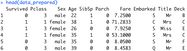
Let’s start by loading the data and displaying the head of the dataset:

data <- get_data()
head(data)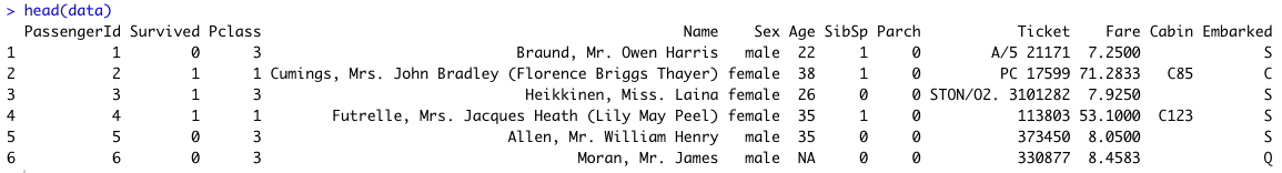

Image 1 – Head of the Titanic dataset

The dataset is quite messy and full of missing values by default. The prepare_data() function is here to fix that:

data_prepared <- prepare_data(data)
head(data_prepared)

Image 2 – Titanic dataset in a machine learning ready form

Next, we’ll split the dataset into training and testing subsets. Once done, the dimensions of both are printed:

data_splitted <- train_test_split(data_prepared)
dim(data_splitted$train_set)
dim(data_splitted$test_set)

Image 3 – Dimensions of training and testing subsets

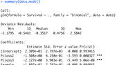
Let’s fit a logistic regression model to the test set and print the model summary:

data_model <- fit_model(data_splitted$train_set)
summary(data_model)

Image 4 – Summary of a logistic regression model

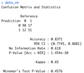
There’s a lot more to the summary, but the important thing is that we don’t get any errors. The final step is to print the confusion matrix:

Eval test:

data_cm <- evaluate_model(data_model, data_splitted$test_set)
data_cm

Image 5 – Model confusion matrix on the test set

And that’s it – everything works, so let’s bring it over to targets next.

Machine Learning Pipeline in R {targets} – Plain English Explanation

By now, you should have a R/functions.R file created and populated with five functions for training and evaluating a logistic regression model.

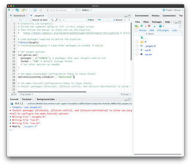
The question remains – How to add these functions to a targets pipeline? The answer is simple, just run the following from the R console:

targets::use_targets()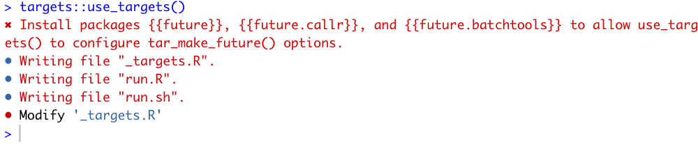

Image 6 – Initializing {targets}

The package will automatically create a new file for you – _targets.R. It’s a normal R script:

Image 7 – _targets.R file

Inside it, you’ll have to modify a couple of things:

• Line 12 – Add all external R packages your script needs.
• Line 28 – Replace the dummy pipeline with the actual one.

Each step of the pipeline has to be placed inside the tar_target() function. The function accepts the step name and the command it will run. Keep in mind that the name isn’t surrounded by quotes, which means you can pass the result of one step to the other.

Here’s the entire modified _targets.R file:

# Created by use_targets().
# Follow the comments below to fill in this target script.
# Then follow the manual to check and run the pipeline:
#   https://books.ropensci.org/targets/walkthrough.html#inspect-the-pipeline # nolint

# Load packages required to define the pipeline:
library(targets)
# library(tarchetypes) # Load other packages as needed. # nolint

# Set target options:
tar_option_set(
  packages = c("tibble", "titanic", "dplyr", "modeest", "mice", "caTools", "caret"), # packages that your targets need to run
  format = "rds" # default storage format
  # Set other options as needed.
)

# tar_make_clustermq() configuration (okay to leave alone):
options(clustermq.scheduler = "multicore")

# tar_make_future() configuration (okay to leave alone):
# Install packages {{future}}, {{future.callr}}, and {{future.batchtools}} to allow use_targets() to configure tar_make_future() options.

# Run the R scripts in the R/ folder with your custom functions:
tar_source()
# source("other_functions.R") # Source other scripts as needed. # nolint

# Replace the target list below with your own:
list(
  tar_target(data, get_data()),
  tar_target(data_prepared, prepare_data(data)),
  tar_target(data_splitted, train_test_split(data_prepared)),
  tar_target(data_model, fit_model(data_splitted$train_set)),
  tar_target(data_cm, evaluate_model(data_model, data_splitted$test_set))
)

That’s all we need to do, preparation-wise. We’ll now check if there are any errors in the pipeline.

Check the pipeline for errors

Each time you write a new pipeline or make changes to an old one, it’s a good idea to check if everything works. That’s where the tar_manifest() function comes in.

You can call it directly from the R console:

targets::tar_manifest(fields = command)

Here’s the output you should see if there are no errors:

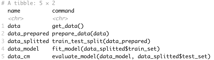
Image 8 – Tar manifest output

The tar_manifest() function is used for creating a manifest file that describes the targets and their dependencies in a computational pipeline. The manifest file serves as a blueprint for the pipeline and guides the execution and management of targets.

Everything looks good here, but that’s not the only check we can do.

R {targets} dependency graph

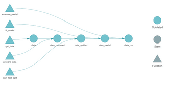
Let’s discuss an additional, more visual test. The tar_visnetwork() function renders the dependency graph which shows a natural progression of the pipeline from left to right.

When you call this function for the first time, you’ll likely be prompted to install the visnetwork library (press 1 on the keyboard):

targets::tar_visnetwork()

Image 9 – {targets} dependency graph

You can clearly see the dependency relationship – the output of each pipeline element is passed as an input to the next element. The functions displayed as triangles on the left are connected with their respective pipeline element.

Next, let’s finally run the pipeline.

Run targets pipeline

Running the pipeline also boils down to calling a single function – tar_make():

targets::tar_make()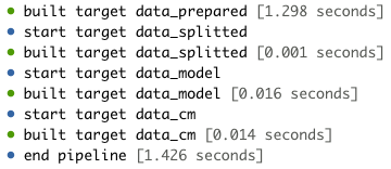

Image 10 – Pipeline progress

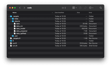
If you don’t see any errors (chunks of red text), it means your pipeline was successfully executed. You should see a new _targets folder created:

Image 11 – Contents of the _targets folder

The _targets/objects is a folder containing the output of each pipeline step. We can load the results of the last step (confusion matrix) and display it in the R console:

targets::tar_read(data_cm)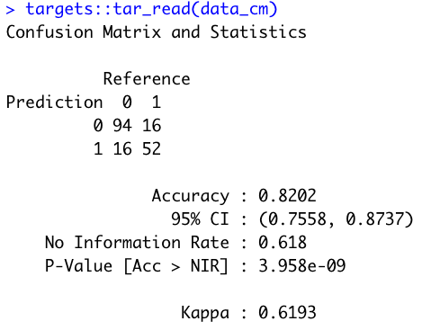

Image 12 – Confusion matrix of a logistic regression model

Yes, it’s that easy! But one of the best targets features is that it won’t run a pipeline step for which either the code or the data haven’t changed. We can verify this by re-running the pipeline:

targets::tar_make()

Image 13 – Pipeline progress – all steps skipped

And that’s the power of the R targets package. Let’s make a short recap next.

Summing up R {targets}

Today you’ve learned the basics of the {targets} package through a hands-on example. You now have a machine learning pipeline you can modify to your liking. For example, you could load the dataset from a file instead of a library, you could plot the confusion matrix, or print variable importance. Basically, there’s no limit to what you can do. The modifications you’d have to make in _targets.R file is minimal, and you can easily figure them out by referencing the documentation.

What’s your favorite approach to writing machine learning pipelines in R? Are you still using the drake package? Please let us know in the comment section below. We also encourage you to move the discussion to Twitter – @appsilon. We’d love to hear your input.

Building a Shiny app for your machine learning project? Add automated validation and implment a CI/CD pipeline with Posit Connect and GitLab-CI.