Guide to GPU-accelerated Ship Recognition in Satellite Imagery Using Keras and R (part II)

23 January 2018

Before we start…

We hope you found the first half of this post useful and interesting. Before we dive into the code, I want to explain a few important aspects of data science. Firstly, implementing data science in practice is always a research process. The goals we set have a significant impact on the methods chosen. Trying to achieve even a marginal increase in accuracy or precision can have a significant impact on the project’s duration. Development is heavily influenced by the data, as well. Achieving the same results on different data sets is not always a straightforward process.

Furthermore, I want to describe why we use GPU’s over CPU’s to train our models. It is important to go into the differences between the two. CPU’s only have a few cores. Generally, each core works on a single process at a time. GPU’s on the other hand, has hundreds of weaker cores.

Technically speaking, training a model is done through thousands of small processes and individual statistical manipulations. Each of these processes can be done at the same time on a GPU, vastly decreasing the necessary time needed for training. The differences are most apparent in Deep Learning.

The data

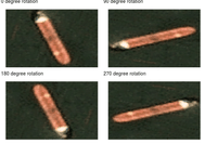
Before we start changing our CNN’s architecture, there are some things we can do when preparing our data. As a reminder, we’ve got 2800 satellite images (80-pixel height, 80-pixel width, 3 colors – RGB color space). This isn’t a huge sample, especially in Deep Learning, but it will do for our needs. In situations like this, a common practice is to use some geometric transformation (rotation, translation, thickening, blurring, etc.) to enlarge the training set. For example, in R we can use the rot90 function from the pracma package to create images rotated by 90, 180, or 270 degrees. We now have to slightly modify the code:

library(keras)
library(tidyverse)
library(jsonlite)
library(abind)
library(gridExtra)
library(pracma)

ships_json <- fromJSON("ships_images/shipsnet.json")[1:2]

ships_data <- ships_json$data %>%
  apply(., 1, function(x) {
    r <- matrix(x[1:6400], 80, 80, byrow = TRUE) / 255
    g <- matrix(x[6401:12800], 80, 80, byrow = TRUE) / 255
    b <- matrix(x[12801:19200], 80, 80, byrow = TRUE) / 255
    list(array(c(r, g, b), dim = c(80, 80, 3)), # Orginal
         array(c(rot90(r, 1), rot90(g, 1), rot90(b, 1)), dim = c(80, 80, 3)), # 90 degrees
         array(c(rot90(r, 2), rot90(g, 2), rot90(b, 2)), dim = c(80, 80, 3)), # 180 degrees
         array(c(rot90(r, 3), rot90(g, 3), rot90(b, 3)), dim = c(80, 80, 3))) # 270 degrees
  }) %>%
  do.call(c, .) %>%
  abind(., along = 4) %>% # Combine 3-dimensional arrays into 4-dimensional array
  aperm(c(4, 1, 2, 3)) # Array transposition

ships_labels <- ships_json$labels %>%
  map(~ rep(.x, 4)) %>%
  unlist() %>%
  to_categorical(2)

set.seed(1234)
indexes <- sample(1:dim(ships_data)[1], 0.7 * dim(ships_data)[1] / 4) %>%
  map(~ .x + 0:3) %>%
  unlist()
train <- list(data = ships_data[indexes, , , ], labels = ships_labels[indexes, ])
test <- list(data = ships_data[-indexes, , , ], labels = ships_labels[-indexes, ])

xy_axis <- data.frame(x = expand.grid(1:80, 80:1)[ ,1],
                      y = expand.grid(1:80, 80:1)[ ,2])

sample_plots <- 1:4 %>% map(~ {
  plot_data <- cbind(xy_axis,
                     r = as.vector(t(ships_data[.x, , ,1])),
                     g = as.vector(t(ships_data[.x, , ,2])),
                     b = as.vector(t(ships_data[.x, , ,3])))
  ggplot(plot_data, aes(x, y, fill = rgb(r, g, b))) +
    guides(fill = FALSE) +
    scale_fill_identity() +
    theme_void() +
    geom_raster(hjust = 0, vjust = 0) +
    ggtitle(paste(((.x - 1) * 90) %% 360, "degree rotation"))
})

do.call("grid.arrange", c(sample_plots, ncol = 2, nrow = 2))

CNN’s architecture

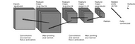
We can change the architecture of our ConvNet in many different ways. The first and simplest thing we can try is to add more layers. Our initial network looks like this:

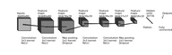
We will add some previously mentioned layers (convolutional, pooling, activation), but can also add some new ones. Our network is getting bigger and more complicated. As such, it could be prone to overfitting. To prevent this we can use a regularization method called dropout. In dropout, individual nodes are either removed from the network with some probability 1-p or kept with probability p. To add dropout to a convolutional neural network in Keras we can use the layer_dropout() function and set the rate parameter to a desired probability. Our example architecture could look like this:

model2 <- keras_model_sequential()
model2 %>%
  layer_conv_2d(
    filter = 32, kernel_size = c(3, 3), padding = "same", 
    input_shape = c(80, 80, 3), activation = "relu") %>%
  layer_conv_2d(filter = 32, kernel_size = c(3, 3),
                activation = "relu") %>%
  layer_max_pooling_2d(pool_size = c(2, 2)) %>%
  layer_dropout(0.25) %>%
  layer_conv_2d(filter = 64, kernel_size = c(3, 3), padding = "same",
                activation = "relu") %>%
  layer_conv_2d(filter = 64, kernel_size = c(3, 3),
                activation = "relu") %>%
  layer_max_pooling_2d(pool_size = c(2, 2)) %>%
  layer_dropout(0.25) %>%
  layer_flatten() %>%
  layer_dense(512, activation = "relu") %>%
  layer_dropout(0.5) %>%
  layer_dense(2, activation = "softmax")

Optimizer

After preparing our training set and setting up the architecture, we can choose a loss function and optimization algorithm. In Keras, you can choose from several algorithms such as a simple Stochastic Gradient Descent to a more adaptive algorithm like Adaptive Moment Estimation. Choosing a good optimizer could be crucial. In Keras, optimizer functions start with optimizer_:

model2 %>% compile(
  loss = "categorical_crossentropy",
  optimizer = optimizer_adamax(lr = 0.0001, decay = 1e-6),
  metrics = "accuracy"
)

Results

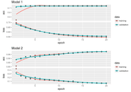
The figure below shows the values of our accuracy and loss function (cross-entropy) before (Model 1) and after (Model 2) modifications. We can see noticeable growth in our validation set accuracy (from 0.7449 to 0.9828) and loss function decrease (from 0.556 to 0.04573).