Introduction to SQL: 5 Key Concepts Every Data Professional Must Know

Introduction to SQL

SQL has been around for decades, and is a go-to language for data analysis and lookups. With the rise of data-related programming languages such as R and Python, it’s easy to use SQL only for a simple SELECT * statement and perform the filterings and aggregations later. While tempting, that’s not the best solution.

Are you a programmer who wants to learn R? Check out our complete R guide for programmers.

Today you’ll learn the basics of SQL through a ton of hands-on examples. You’ll need to have a PostgreSQL database installed to follow along.

The article is structured as follows:

• Dataset introduction
• Select data
• Filter data
• Sort data
• Match data
• Join and group data
• Conclusion

Dataset Introduction

As briefly mentioned earlier, you’ll need to have the PostgreSQL database installed. You’ll also need the Dvd Rental dataset that you can load to your database via the restore functionality.

The ER diagram of the Dvd rental dataset is shown below:

Image 1 – DVD rental database diagram (source: https://www.postgresqltutorial.com/postgresql-sample-database/)

You’ll use customer and payment tables throughout the article, but feel free to explore the others on your own.

Select Data

The most basic operation you’ll do with SQL is selecting the data. It’s done with the SELECT keyword (not case-sensitive). If you want to grab all columns from a particular table, you can use the SELECT * FROM <table_name> syntax. Likewise, if you want only specific columns, you can replace the star sign with column names.

Let’s take a look at a couple of examples to grasp a full picture.

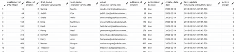
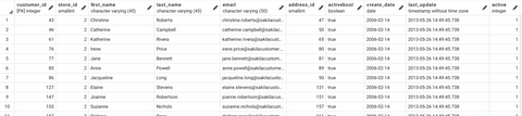
Here’s how you can grab all data from the customer table:

The results are shown in the image below:

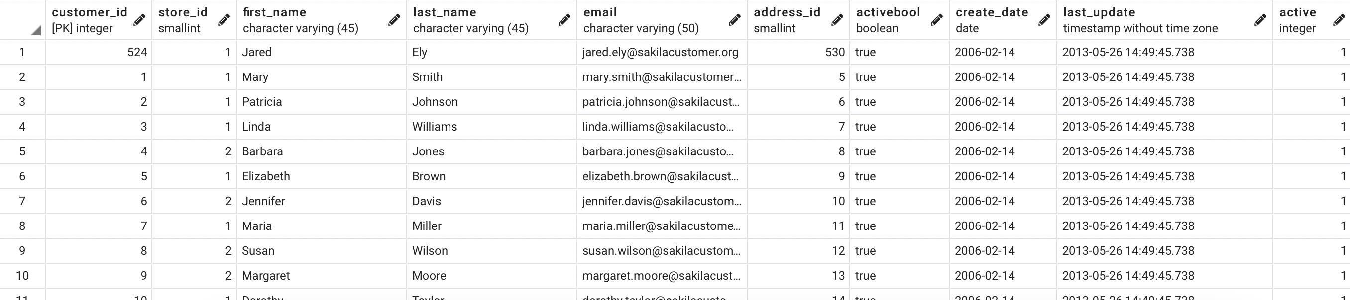
Image 2 – Data from the customer table

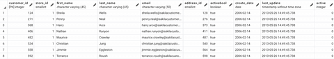
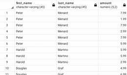
But what if you only want the data on customer ID, first, and last name? Here’s what you can do:

And here are the results:

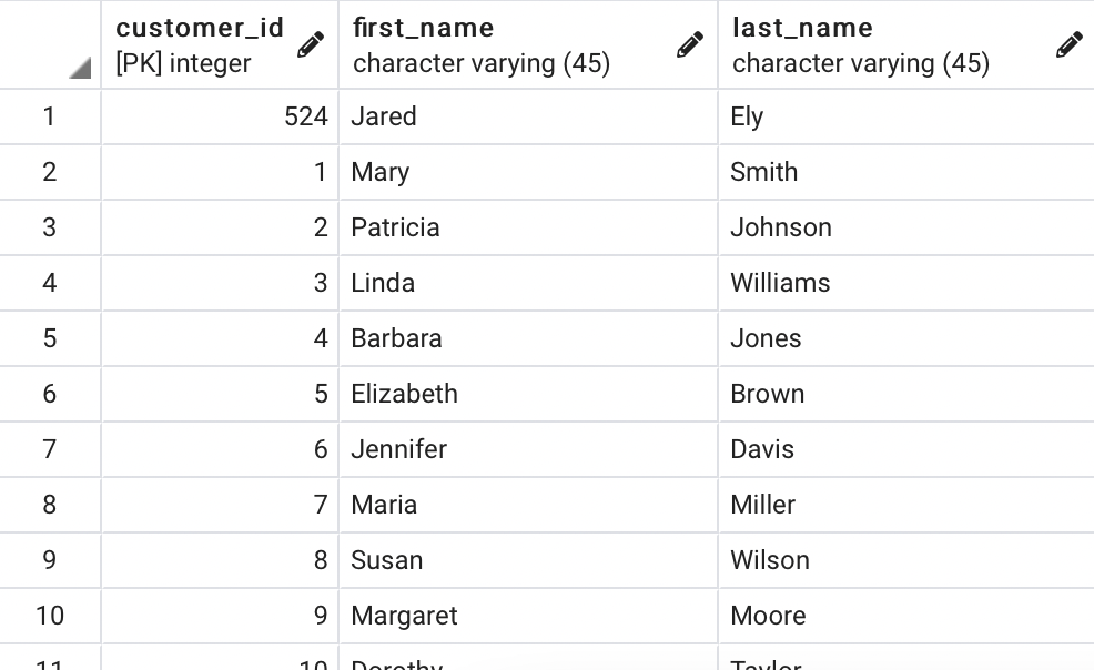
Image 3 – Data from the customer table – custom columns

It’s always a good practice to specify column names instead of using the star syntax. The table structure might change in the future, so you might end up with more columns than anticipated. Even if that’s not the case, what’s the point of selecting columns you won’t work with?

Filter Data

It’s highly likely you won’t need all records from a table. That’s where filtering comes into play. You can filter the result set with the WHERE keyword. Any condition that has to be met goes after it.

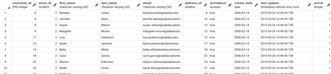
Here’s how you can grab only inactive customers:

The results are shown below:

Image 4 – Inactive customers from the customer table

But what if you want to filter by multiple conditions? You can’t use the WHERE keyword again. Instead, you can list conditions separated by the AND keyword.

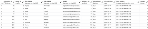
Here’s how to select all inactive customers from the first store (store_id is 1):

Here are the results:

Image 5 – Inactive customers from the first store

You can put as many filter conditions after this one; just make sure to separate them with the AND keyword.

Sort Data

Sorting is an essential part of every analysis. Maybe you want to sort users by their registration date, products by the expiration date, or movies by rating – the ORDER BY keyword has you covered.

Let’s see how you can sort the customers by their respective ID:

The results are shown below:

Image 6 – Customers sorted by the customer ID

As you can see, sorting works in ascending order by default. Sometimes you want items ordered from highest to lowest (descending), so you’ll need one additional keyword – DESC.

Here’s how to do the same sorting but in descending order:

The results are shown in the image below:

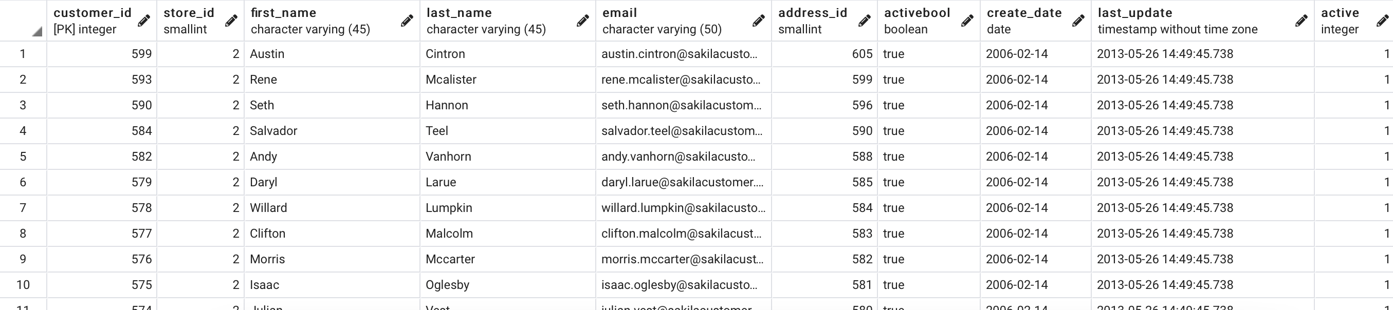
Image 7 – Customers sorted by customer ID in the descending order

And that’s all there is to data sorting.

Match Data

Sometimes you don’t know what exactly are you looking for, but you have a rough idea. For example, maybe you know that the name of the customer of interest starts with some letter (or a sequence of letters), but you’re not quite sure.

That’s where matching comes in. In SQL, matching is implemented with the LIKE keywords. There are multiple ways to do matching, but we’ll cover only the basics.

For example, let’s say you want to see only these customers whose first name starts with “An”:

The results are shown below:

Image 8 – Customers whose first name starts with “An”

You can do matching on different parts of the variable. For example, let’s say you want only those customers whose first name ends with “ne”:

Here are the results:

Image 9 – Customers whose first name ends with “ne”

There are more advanced matching operations, like specifying the number of characters before and after, but that’s beyond the scope for today.

Join and Group Data

It’s improbable that all of the data you need is stored in a single table. More often than not, you’ll have to use joins to combine results from two or more tables. Luckily, that’s easy to do with SQL.

There are many types of joins:

• INNER JOIN – returns the rows that have matching values in both tables
• LEFT JOIN – returns all rows from the left table and only the matched rows from the right table
• RIGHT JOIN – returns all rows from the right table and only the matched rows from the left table
• FULL JOIN – returns all rows when there’s a match in either table

Here’s how you can use joins to combine customer and payment tables and extract the amount paid per transaction:

The results are shown below:

Image 10 – Amount paid per transaction by a customer

As you can see, there are multiple records for every customer. That’s because a single record represents a single transaction, and a single customer can make multiple transactions.

If you want to find the sum of the amounts for every customer, you’ll have to use the GROUP BY keyword and an aggregation function. Let’s take a look at an example:

The results are shown below:

Image 11 – Total amount per customer

So what happened here? Put simply, you’ve made distinct groups from every first and last name (and assumed every customer has a unique name) and calculated the sum per group.

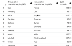
A couple of things can be improved. For example, right now we’re returning all records completely unsorted. The following code snippet orders the rows by the total sum (descending) and keeps only the first five rows:

Here are the results:

Image 12 – Top 5 customers by the amount spent

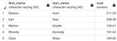
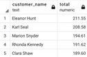
You can still improve this result set. For example, let’s say you want to combine the first and last name to a single column named customer_name, and you also want to rename the aggregated column to total:

The results are shown below:

Image 13 – Top 5 customers by the amount spent (v2)

Conclusion

Today you’ve learned the basics of SQL in the PostgreSQL environment. SQL is a broad topic, and you can (and should) always learn more. More intermediate and advanced-level guides are coming soon, so stay tuned to the Appsilon blog.

To summarize – do as much data filtering/aggregating in the database. It’s a much faster approach than dragging the entire dataset(s) to the memory and performing the filtering there.

Learn More

• 7 Must-Have Skills to Get a Job as a Data Scientist
• Machine Learning with R: A Complete Guide to Linear Regression
• Machine Learning with R: A Complete Guide to Logistic Regression
• How to Make REST APIs with R: A Beginners Guide to Plumber
• How to Analyze Data with R: A Complete Beginner Guide to dplyr

Appsilon is hiring for remote roles! See our Careers page for all open positions, including R Shiny Developers, Fullstack Engineers, Frontend Engineers, a Senior Infrastructure Engineer, and a Community Manager. Join Appsilon and work on groundbreaking projects with the world’s most influential Fortune 500 companies.