Beyond Equality: Unleashing the Power of Non-Equi Joins in {dplyr}

R, a language renowned for its data analysis capabilities, is embraced by data scientists worldwide. Within the expansive realm of R packages, the Tidyverse ecosystem stands out as a powerful and cohesive toolkit for data manipulation and visualization.

In this comprehensive exploration, we’ll dive into the capabilities of {dplyr}, a core component of the Tidyverse, and unveil the magic of non-equi joins and rolling joins within this tidy framework. These advanced functionalities not only enhance the expressiveness of your analyses but also seamlessly integrate into the philosophy of tidy data, considerably reducing the cognitive bottleneck.

Looking to enhance your R skills with the power of {dplyr}? Discover the essentials in our easy-to-follow blog post, How to Analyze Data with R: A Complete Beginner Guide to dplyr.

Table of Contents

• The Elegance of Non-Equi Joins in {dplyr}
• The R Ecosystem and Non-Equi Joins
• Scenario 1: Exploring Patient Medication Usage
• Scenario 2: Analyzing Temporal Relationships of Ship Arrivals
• Conclusion: A Tidy Symphony of Power and Precision

The Elegance of Non-Equi Joins in {dplyr}

Traditional joins in databases often revolve around equality conditions. However, in real-world scenarios, relationships between datasets can be more intricate. With its clean syntax, non-equi joins are one of the most recent significant additions to {dplyr} (>= 1.1.0). They provide a sophisticated way to overcome the constraints of basic equality requirements.

The R Ecosystem and Non-Equi Joins

When it comes to data analysis, flexibility is key, and for non-equi joins there are various tools at your disposal. In R, the {data.table} package provides a robust solution, allowing for efficient data manipulation. Alternatively, using {DBI} you can connect to a range of different databases, from the simple and time-tested SQLite, to more modern options like DuckDB. Whether you choose the convenience and expressiveness of {dplyr}, the minimal syntax and speed of {data.table}, or the structured querying power of databases, the versatility of non-equi joins remains a valuable asset in your data analysis toolkit in all these approaches.

Seeking the fastest way to perform data lookups in R? Compare dplyr vs data.table in our insightful blog post.

Scenario 1: Exploring Patient Medication Usage

In the dynamic landscape of healthcare data analysis, understanding the correlation between patient admissions and medication prescriptions is pivotal for delivering effective patient care. In this example, we delve into the practical application of the {dplyr} package in R to conduct a non-equi join, shedding light on patients who were admitted to a hospital while they were on medication.

Setting the Stage

Our journey begins by crafting two straightforward datasets: one encapsulating patient information and admission dates and the other detailing medication prescriptions.

Execute the subsequent code to generate these datasets:

library(dplyr)

# Creating a tibble for patients and admissions
patients <- tibble(
  patient_id = c(1, 2, 3),
  patient_name = c("Alice", "Bob", "Charlie"),
  admission_date = as.Date(c("2022-01-01", "2022-02-15", "2022-03-10"))
)

# Creating a tibble for medication prescriptions
medications <- tibble(
  patient_id = c(1, 1, 2, 3, 3),
  medication_name = c("Aspirin", "Tylenol", "Ibuprofen", "Amoxicillin", "Vitamin C"),
  start_date = as.Date(c("2021-12-01", "2022-02-01", "2022-02-20", "2022-01-15", "2022-04-01")),
  end_date = as.Date(c("2022-01-31", "2022-02-28", "2022-03-15", "2022-02-28", "2022-04-30"))
)

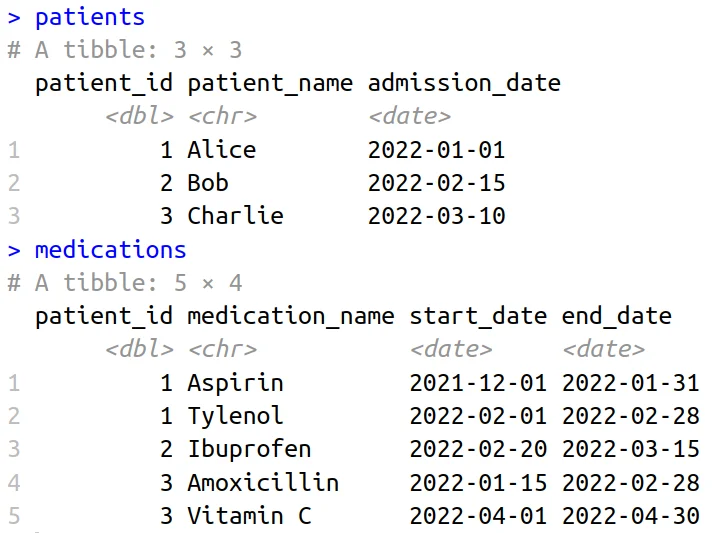
Patient Admission and Medication Tables

Unveiling Patient-Medication Relationships

Now, let’s harness the capabilities of {dplyr} to unravel patient-medication relationships through a non-equi join:

# Performing non-equi join
result <- patients |>
 inner_join(
   medications,
   by = join_by(
     patient_id,
     admission_date >= start_date,
     admission_date <= end_date
   )
 )

This is a special case of non-equi join called overlap join. Using some of {dplyr}’s syntactic sugar we can rewrite it in a more readable way:

# Equivalent overlap join
result <- patients |>
  inner_join(
    medications,
    by = join_by(
      patient_id,
      between(admission_date, start_date, end_date)
    )
  )

resulting in:

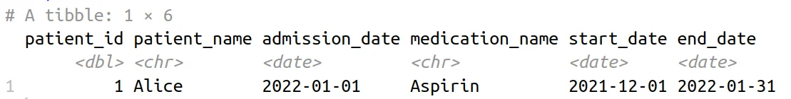
Patient Medication Record Table

In this example, the inner_join() function, coupled with the join_by() helper, defines the conditions for the non-equi join. We’re matching patient_id and checking whether the admission_date falls within the start_date and end_date range for each medication prescription.

The resultant table gives us insight into patients who were admitted to a hospital while they were on medication. This includes comprehensive details such as patient information, admission dates, prescribed medications, and the corresponding start and end dates of the prescriptions. Non-equi joins in {dplyr} provide an intuitive and robust approach to analyzing temporal relationships in healthcare data.

Scenario 2: Analyzing Temporal Relationships of Ship Arrivals

Predicting the arrival time of ships at a port is a common scenario in maritime logistics and supply chain management. Non-equi joins are one way to analyze historical data and derive insights that can help for example to predict the next ship’s arrival time. In this example, we’ll illustrate non-equi and rolling joins that are useful for temporal analysis in shipping.

Setting the Stage

Consider a scenario where we have a dataset named ships containing information about ships arriving at ports, including the ship’s unique identifier (ship_id), the arrival timestamp (arrival_time), and departure time (departure_time).

library(dplyr)

ships <- tibble(
  ship_id = 1:4,
  arrival_time = as.POSIXct(c(
    "2022-01-01 18:00:00",
    "2022-01-01 21:30:00",
    "2022-01-02 02:45:00",
    "2022-01-02 15:15:00"
  )),
  departure_time = as.POSIXct(c(
    "2022-01-01 22:00:00",
    "2022-01-02 03:30:00",
    "2022-01-02 05:45:00",
    "2022-01-02 18:15:00"
  ))
)

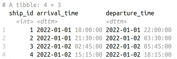
Shipping Schedule Data Table

Setting Up a Non-Equi Join

Now, let’s set up a scenario where we want to identify vessels with port stay overlap. We can achieve this using a self-non-equi join using overlaps() within the join_by() function call:

ships |>
  inner_join(
    ships,
    by = join_by(
      x$ship_id < y$ship_id, # Only consider ordered pairs
      overlaps(
        x_lower = x$arrival_time,
        x_upper = x$departure_time,
        y_lower = y$arrival_time,
        y_upper = y$departure_time
      )
    )
  )

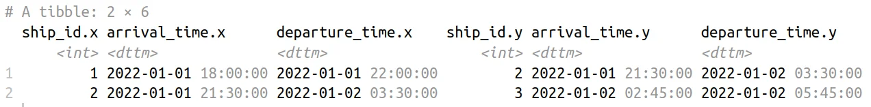
Comparative Ship Scheduling Data Table

We employed the inner_join() function to identify pairs of ships that have overlapping time intervals during their presence at the port. The join_by() function is used to filter the pairs based on the condition that the ship_id of the first ship (x) should be less than the ship_id of the second ship (y), ensuring only ordered pairs are considered.

The overlaps() function within join_by() checks for time overlaps between the arrival and departure intervals of the two ships. In summary, the code identifies and outputs pairs of ships that arrived at the port during overlapping time periods, providing insights into potential interactions or congestion scenarios in the port schedule.

Setting Sail with a Rolling Join

Let’s extend our scenario further. Suppose that we have information about cargo readiness, detailing when cargoes are prepared for shipment, and the dataset of ships from the previous section.

cargoes <- tibble(
  cargo_id = 1:4,
  ready_for_shipment = as.POSIXct(c(
    "2022-01-01 10:00:00",
    "2022-01-01 11:00:00",
    "2022-01-01 20:00:00",
    "2022-01-02 10:00:00"
  ))
)

Suppose that we want for each cargo to find a ship that can depart with it as soon as possible.

We can seamlessly blend the cargoes and ships datasets using a special class of non-equi joins called rolling-joins. Rolling joins are activated by wrapping an inequality in closest().

This approach allows us to consider the temporal relationship between cargo readiness and ship arrivals under a constraint.

cargoes |> 
  left_join(
    ships,
    by = join_by(closest(ready_for_shipment < departure_time))
  )

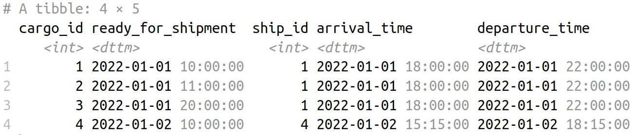
Cargo and Shipping Schedule Table

In the above code example, join_by(closest(ready_for_shipment < departure_time)) ensures that we join the datasets based on the condition that the departure time is after the cargo is ready for shipment. In addition, the closest() function call in join_by() will “roll” the ship with the earliest departure time to cargoes.

Put another way, we join under the condition ready_for_shipment < departure_time, but we filter down the results so that for each ready_for_shipment time, we keep the ship with the closest possible departure time. This creates a harmonious union of cargo and ship data, setting the stage for more nuanced analysis.

Wondering how to supercharge your R data processing without major code revisions? Dive into R Data Processing Frameworks: How To Speed Up Your Data Processing Pipelines up to 20 Times.

Conclusion: A Tidy Symphony of Power and Precision

As datasets grow in complexity and size, the need for tools that combine efficiency with versatility becomes paramount. {dplyr}, as part of the Tidyverse, stands out as a robust solution, providing a seamless blend of efficiency and functionality.

In scenarios where intricate relationships between numerical variables arise, non-equi joins are powerful and versatile tools. The tidy syntax ensures that our code remains readable and consistent, aligning with the principles of tidy data. Whether navigating financial markets, healthcare data, deciphering sales trends, or managing complex event timelines, the power of {dplyr} shines through. Happy coding, and may your data explorations be insightful and efficient with the power of the Tidyverse!

Did you find this blog post useful? Learn more about the beauty of writing clearer, more intuitive code and the advantages of using {dplyr} in our Functional Programming in R ebook.