Deep Learning with R and Keras: Build a Handwritten Digit Classifier in 10 Minutes

Dario Radečić

25 February 2021

Updated: December 30, 2022.

Deep Learning in R – MNIST Classifier with R Keras

In a day and age where everyone seems to know how to solve at least basic deep learning tasks with Python, one question arises: How does R fit into the whole deep learning picture?

You don’t need deep learning algorithms to solve basic image classification tasks. Here’s how to classify handwritten digits with R and Random Forests.

Here is some good news for R fans – both Tensorflow and Keras libraries are available to you, and they’re easy to configure. Today you’ll learn how to solve a well-known MNIST problem with Keras.

Navigate to a section:

Installing Tensorflow and Keras with R
Dataset Loading and Preparation
Model Training
Model Evaluation
Conclusion

Installing Tensorflow and Keras with R

To build an image classifier model with Keras, you’ll have to install the library first. But before you can install Keras, you’ll have to install Tensorflow.

The procedure is a bit different than when installing other libraries. Yes, you’ll still use the install.packages() function, but there’s an extra step involved.

Here’s how to install Tensorflow from the R console:

install.packages("tensorflow")
library(tensorflow)
install_tensorflow()

Most likely, you’ll be prompted to install Miniconda, which is something you should do – assuming you don’t have it already.

The installation process for Keras is identical – just be aware that Tensorflow has to be installed first:

install.packages("keras")
library(keras)
install_keras()

Restart the R session if you’re asked to – failing to do so could result in some DLL issues, at least according to R.

And that’s all you need to install the libraries. Let’s load and prepare the dataset next.

Dataset Loading and Preparation

Luckily for us, the MNIST dataset is built into the Keras library. You can get it by calling the dataset_mnist() function once the library is imported.

Further, you should separate the dataset into four categories:

X_train – contains digits for the training set
X_test – contains digits for the testing set
y_train – contains labels for the training set
y_test – contains labels for the testing set

You can use the following code snippet to import Keras and unpack the data:

library(keras)

mnist <- dataset_mnist()
X_train <- mnist$train$x
X_test <- mnist$test$x
y_train <- mnist$train$y
y_test <- mnist$test$y

It’s a good start, but we’re not done yet. This article will only use linear layers (no convolutions), so you’ll have to reshape the input images from 28×28 to 1×784 each. You can do so with the array_reshape() function from Keras. Further, you’ll also divide each value of the image matrix by 255, so all images are in the [0, 1] range.

That will handle the input images, but we also have to convert the labels. These are stored as integers by default, and we’ll convert them to categories with the to_categorical() function.

Here’s the entire code snippet:

X_train <- array_reshape(X_train, c(nrow(X_train), 784))
X_train <- X_train / 255

X_test <- array_reshape(X_test, c(nrow(X_test), 784))
X_test <- X_test / 255

y_train <- to_categorical(y_train, num_classes = 10)
y_test <- to_categorical(y_test, num_classes = 10)

And that’s all we need to start with model training. Let’s do that next.

Model Training

MNIST is a large and simple dataset, so a simple model architecture should result in a near-perfect model.

We’ll have three hidden layers with 256, 128, and 64 neurons, respectively, and an output layer with ten neurons since there are ten distinct classes in the MNIST dataset.

Every linear layer is followed by dropout in order to prevent overfitting.

Once you declare the model, you can use the summary() function to print its architecture:

model <- keras_model_sequential() %>%
  layer_dense(units = 256, activation = "relu", input_shape = c(784)) %>%
  layer_dropout(rate = 0.25) %>% 
  layer_dense(units = 128, activation = "relu") %>%
  layer_dropout(rate = 0.25) %>% 
  layer_dense(units = 64, activation = "relu") %>%
  layer_dropout(rate = 0.25) %>%
  layer_dense(units = 10, activation = "softmax")
summary(model)

The results are shown in the following figure:

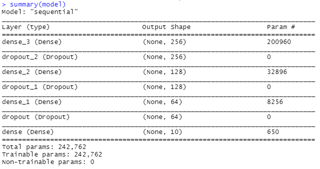
Image 1 – Summary of our neural network architecture

One step remains before we can begin training – compiling the model. This step involves choosing how loss is measured, choosing a function for reducing loss, and choosing a metric that measures overall performance.

Let’s go with categorical cross-entropy, Adam, and accuracy, respectively:

model %>% compile(
  loss = "categorical_crossentropy",
  optimizer = optimizer_adam(),
  metrics = c("accuracy")
)

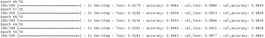
You can now call the fit() function to train the model. The following snippet trains the model for 50 epochs, feeding 128 images at a time:

history <- model %>% 
  fit(X_train, y_train, epochs = 50, batch_size = 128, validation_split = 0.15)

Once this line of code is executed, you’ll see the following output:

Image 2 – Model training (step 1)

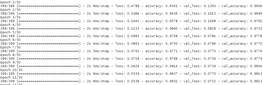
After a minute or soo, 50 epochs will elapse. Here’s the final output you should see:

Image 3 – Model training (step 2)

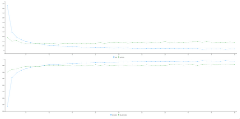
At the same time, you’ll see a chart updating as the model trains. It shows both loss and accuracy on training and validation subsets. Here’s how it should look like when the training process is complete:

Image 4 – Loss and accuracy on training and validation sets

And that’s it – you’re ready to evaluate the model. Let’s do that next.

Model Evaluation

You can use the evaluate() function from Keras to evaluate the performance on the test set. Here’s the code snippet for doing so:

model %>%
  evaluate(X_test, y_test)

And here are the results:

Image 5 – Model evaluation on the test set

As you can see, the model resulted in an above 98% accuracy on previously unseen data.

To make predictions on a new subset of data, you can use the predict_classes() function as shown below (UPDATE 2022: make sure to add k_argmax() to the end because the old way doesn’t work anymore):

predictions <- model %>%
  predict(X_test) %>%
  k_argmax()

predictions$numpy()

Here are the results:

Image 6 – Class predictions on the test set

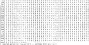
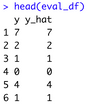
You can take the R Keras model evaluation to the next step by creating a custom evaluation dataframe object. The one below contains actual test values and predictions. Keep in mind that a constant number 1 is subtracted from the actual value to get numbers in range between 0 and 9 instead of 1 to 10:

library(ramify)

eval_df <- data.frame(
  y = argmax(y_test),
  y_hat = predictions$numpy()
)
eval_df$y <- lapply(eval_df$y, function(x) x - 1)

head(eval_df)

Image 7 – Head of the evaluation data.frame

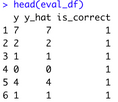
You can now further feature engineer attributes as you wish. For example, here’s how you can add a column which compares the two existing ones to see if classification is correct:

eval_df$is_correct <- ifelse(eval_df$y == eval_df$y_hat, 1, 0)

head(eval_df)

Image 8 – Head of the evaluation data.frame (2)

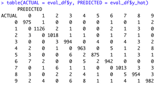
Probably the biggest reason you’d want a custom evaluation dataframe is so you can calculate custom evaluation metrics. For example, the dataframe has to be unlisted before you can construct a confusion matrix:

eval_df <- as.data.frame(lapply(eval_df, unlist))
table(ACTUAL = eval_df$y, PREDICTED = eval_df$y_hat)

Image 9 – MNIST confusion matrix

MNIST is a 10-class classification problem, so the confusion matrix isn’t so easy to look at. Calculating metrics such as precision and recall is also challenging due to the number of classes.

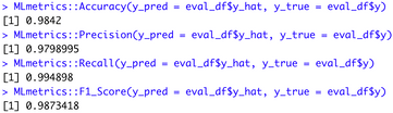
Luckily, you can use dedicated R packages to calculate these metrics easily:

library(MLmetrics)

MLmetrics::Accuracy(y_pred = eval_df$y_hat, y_true = eval_df$y)
MLmetrics::Precision(y_pred = eval_df$y_hat, y_true = eval_df$y)
MLmetrics::Recall(y_pred = eval_df$y_hat, y_true = eval_df$y)
MLmetrics::F1_Score(y_pred = eval_df$y_hat, y_true = eval_df$y)

Image 10 – Test set metrics

And that’s how you can use Keras in R! Let’s wrap things up in the next section.

Summing up R Keras

Most of the online resources for deep learning are written in R – I’ll give you that. That doesn’t mean R is obsolete in this area. Both Tensorflow and Keras have official R support, and model development is just as easy as with Python.

If you want to implement machine learning in your organization, you can always reach out to Appsilon for help.