Introduction to Transfer Learning: Effective Machine Learning Without Custom Architecture

What is Transfer Learning?

Transfer Learning (TL) is one of the most powerful methods for building high-performance deep learning models in computer vision. TL is based on the knowledge-reusability concept – one can use knowledge from one area and apply it to another. By leveraging previous experience, you don’t need to start from scratch with every new model or new situation. So effectively, you can learn how to do new tasks more efficiently by drawing on previous knowledge. 

• Transfer Learning Workflow
• Example: Classification with a Custom Network
• Example: Transfer Learning 
• Conclusion

New to deep learning? Check out our Introduction to Convolutional Neural Networks.

Transfer Learning Workflow

Let’s say you are a data scientist proficient in Python, and now you need to perform a new analysis using R. R might be a new programming language for you. Still, since you already know Python, learning R will be much easier for you compared to a version of yourself that doesn’t know how to program at all. R is a new language, but many of the same principles and fundamentals apply to both Python and R, so you can transfer some of your existing Python knowledge to get a headstart in your pursuit of learning R.

The same principle is used in deep learning with Transfer Learning. Instead of starting from scratch (model with random weights), you can take an existing network that has been trained to do a thing X and customize the network to your particular problem or task. If you read our article on Convolutional Neural Networks (CNNs), then you know that the deeper we go into a network, the more sophisticated are the features that get extracted.

Now imagine that you want to detect dogs and cats in a collection of images. Here’s a 4 step solution for this type of task:

1. We take a network which is very good at detecting objects and customize it. In other words, we take a pre-trained model, e.g., ResNet trained on ImageNet. The existing network’s starting layers focus on detecting ears, eyes, or fur, which will help detect cats and dogs. 
2. We then cut the last few layers (called the head) specialized in a particular task and replace it with a fully connected layer or a few random layers. 
3. Next, we fine-tune the added final layers by training the network on the set of images relevant to our problem (containing cats and dogs). The weights in the initial layers (called the body) won’t get updated (the layers are frozen).
4. Optionally, after fine-tuning the head, we can unfreeze the whole network and train a model a bit more, allowing for weight updates through the entire network.

The advantages of Transfer Learning are faster training and better results with significantly less data.

Example: Classification With a Custom Network

To start, let’s download the Dogs and Cats dataset (link below) from the web and untar the file. We’re doing this task in Google Colab on a Tesla T4 GPU, so your download and training times may vary. Here are the library imports and device configuration: 

import os
import numpy as np
import pandas as pd
import matplotlib.pyplot as plt
from datetime import datetime, timedelta

import torch
import torch.nn as nn
import torch.nn.functional as F
from torch.utils.data import DataLoader
from torchvision.utils import make_grid
from torchvision import models, transforms, datasets

device = torch.device('cuda:0' if torch.cuda.is_available() else 'cpu')

Now we can download the dataset and unpack it:

%mkdir data
%cd /content/data/
!wget http://files.fast.ai/data/examples/dogscats.tgz

!tar zxvf dogscats.tgz

Libraries like PyTorch allow us to enlarge the training data’s size without acquiring more images by performing operations such as rotations and horizontal flips. Further, we’ll prepare every image in the same way (resizing is optional):

• Resize to 224×224 
• Transform from matrix to tensor
• Normalize RGB color channels 

This is performed both for training and testing images, as we essentially want them in the same format. Here’s the code snippet:

DIR_DATA = '/content/data/dogscats/'

train_transforms = transforms.Compose([
    transforms.RandomRotation(10),
    transforms.RandomHorizontalFlip(p=0.5),
    transforms.Resize(224),
    transforms.CenterCrop((224, 224)),
    transforms.ToTensor(),
    transforms.Normalize(
        mean=[0.485, 0.456, 0.406],
        std=[0.229, 0.224, 0.225]
    )
])

valid_transforms = transforms.Compose([
    transforms.Resize(224),
    transforms.CenterCrop((224, 224)),
    transforms.ToTensor(),
    transforms.Normalize(
        mean=[0.485, 0.456, 0.406],
        std=[0.229, 0.224, 0.225]
    )
])

We can now apply the transformation to the images and load them in batches with a PyTorch.DataLoader module. Feel free to experiment with the actual batch size, but we’ve set it to 32 for this case.

train_data = datasets.ImageFolder(os.path.join(DIR_DATA, 'train'), transform=train_transforms)
valid_data = datasets.ImageFolder(os.path.join(DIR_DATA, 'valid'), transform=valid_transforms)

torch.manual_seed(42)
train_loader = DataLoader(train_data, batch_size=32, shuffle=True)
valid_loader = DataLoader(valid_data, batch_size=32, shuffle=False)
class_names = train_data.classes

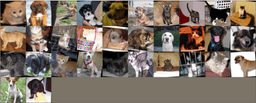
We can now use the declared train_loader to see if transformations were applied. With the help of the matplotlib library, we can visualize the entire batch (32 images):

Judging by the rotation in the images, we can say that everything works as expected up to this point. The next step is to define the neural network class. We decided to go simple, with three convolutional layers, a fully connected layer, and the output layer. Max pooling operation is performed after every convolutional layer, alongside with the ReLU activation. Here’s the model class:

class MyCNN(nn.Module):
    def __init__(self):
        super().__init__()
        self.conv1 = nn.Conv2d(in_channels=3, out_channels=32, kernel_size=3, stride=1)
        self.conv2 = nn.Conv2d(in_channels=32, out_channels=64, kernel_size=3, stride=1)
        self.conv3 = nn.Conv2d(in_channels=64, out_channels=128, kernel_size=3, stride=1)
        self.fc1 = nn.Linear(in_features=26*26*128, out_features=128)
        self.out = nn.Linear(in_features=128, out_features=2)
    
    def forward(self, x):
        x = F.relu(self.conv1(x))
        x = F.max_pool2d(x, kernel_size=2, stride=2)
        x = F.relu(self.conv2(x))
        x = F.max_pool2d(x, kernel_size=2, stride=2)
        x = F.relu(self.conv3(x))
        x = F.max_pool2d(x, kernel_size=2, stride=2)
        x = x.view(-1, 26*26*128)
        x = F.relu(self.fc1(x))
        x = F.dropout(x, p=0.2)
        return self.out(x)

torch.manual_seed(42)

model = MyCNN()
model.to(device)
criterion = nn.CrossEntropyLoss()
optimizer = torch.optim.Adam(model.parameters(), lr=0.001)

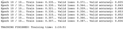
As you can see, the model was moved to the GPU. The model training took around an hour and ten minutes to complete for 10 epochs, and resulted in an 84% accuracy:

Not a bad result for a simple network like this, but can we do better? Transfer learning says yes.

PP-YOLO Object Detection: Why It’s Faster Than YOLOv4

Example: Transfer Learning

The transfer learning approach will be much more straightforward than the custom one. Here are the steps:

1. Download a pretrained network – ResNet with 101 layers will do just fine
2. Freeze the parameters of the pretrained network
3. Update the output layer – as it predicts for 1000 classes and we only have two (dogs and cats) 
4. Transfer the model to the GPU (no pun intended) 
5. Define criterion and optimizer

We can do that in a couple of lines of code:

pretrained_model = models.resnet101(pretrained=True)
for param in pretrained_model.parameters():
    param.requires_grad = False

nb_features = pretrained_model.fc.in_features 

pretrained_model.fc = nn.Linear(nb_features, 2)
pretrained_model.to(device)

pretrained_criterion = nn.CrossEntropyLoss()
pretrained_optimizer = torch.optim.Adam(pretrained_model.fc.parameters(), lr=0.001)

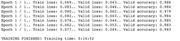
And that’s it! We can start the training process now. It took only 15 minutes for a single epoch and yielded far greater accuracy than our custom architecture:

Now you see how powerful Transfer Learning can be. The existence of Transfer Learning means that custom architectures are obsolete in many cases. 

Conclusion

This article’s take-home point is that stressing out about layers in custom neural network architectures is a waste of time in most cases. Pretrained networks are far more powerful than anything you can come up with on your own in any reasonable amount of time. 

The transfer learning approach requires fewer data and fewer epochs (less training time), so it’s a win-win situation. To be more precise, transfer learning requires more training time per epochs but requires fewer epochs to train a usable model.

If your company needs help with Transfer Learning or you need help with a custom Machine Learning model, reach out to Appsilon. We are experts in Machine Learning and Computer Vision.